Chapter 3 The law of mass action: animals collide

Infectious diseases have been an unpleasant companion of humankind for millions of years. Yet, crowd epidemic diseases could have only emerged within the past 11,000 years, following the rise of agriculture. The ability to maintain large and dense human populations, as well as the close contact with domestic animals, allowed the most deadly diseases to be sustained unlike when human populations were sparse [135].

Perhaps the most-well documented epidemic outbreak in ancient times is the plague of Athens (430-427 BCE) that caused the death of Pericles and killed around 30% of Athens population [136]. The fact that some diseases were contagious was probably well-known way before that. For instance, it has been claimed that in the 14th century BCE the Hittites sent rams infected with tularemia to their enemies to weaken them [137] and there are evidences of quarantine-like isolation of leprous individuals in the Biblical book of Leviticus. Yet, it was thought that diseases were caused by miasma or “bad air” for over 2,000 years. It was not until the end of the XIX century that it was finally discovered that microorganisms were the cause of diseases [138].

The advent of modern epidemiology is usually attributed to John Snow who in the mid of the XIX century traced back the origin of a cholera epidemic in the city of London [139]. However, mathematical methods were not firmly introduced until the beginning of the XX century⁸. Already in 1906 Hamer showed that “an epidemic outbreak could come to an end despite the existence of large numbers of susceptible persons in the population, merely on a mechanical theory of numbers and density” [142]. Although it was thanks to the works by Ross, Kermack and McKendrick that finally a mechanistic theory of epidemics was developed as an analogy to the law of mass-action. In particular, it was McKendrick who gave the title to this chapter when he said in a lecture in 1912: “consider a type of epidemic which is spread by simple contact from human being to human being […] The rate at which this epidemic will spread depends obviously on the number of infected animals, and also on the number of animals that remain to be infected - in other words the occurence of a new infection depends on a collision between an infected and uninfected animal” [143].

The next 50 years were mostly devoted to establishing the mathematical foundations of epidemiology. The problem was that this process was mostly done by mathematicians and statisticians, who were more interested in the theoretical implications of the models rather than in their application to data [144]. This situation changed during the 1980s when Anderson and May, coming from a background in zoology and ecology respectively, started to collaborate with biologists and mathematicians, bridging the gap between data and theory [62]. During the 1990s graphs where introduced in epidemiological models, challenging the classical assumption of homogeneous mixing (that we will discuss in section 3.1), and brought physicists into the field attracted by the similarity of some concepts with phase transitions in non-equilibrium systems [145].

The latest developments of epidemic modeling are based on incorporating more and more data. For instance, the Global Epidemic and Mobility (GLEaM) framework incorporates demographic data of the whole world with short-range and long-range mobility data as the basis of its epidemic model, allowing for the simulation of world-wide pandemics [146]. Similarly, to properly study the spreading of Zika virus it is necessary to take into account the dynamics of mosquitoes, temperature, demographics and mobility, attached to the disease dynamics of the own virus [147]. Multiple sources of data are also being used in the study of vaccination, either to devise efficient administration strategies, including economic considerations [148], or to properly understand how they actually work [149]. Even more, of particular interest nowadays is analyzing the interplay between processes that have been deeply studied in complex systems such as game theory, behavior diffusion and epidemic processes.

Herd immunity, a term coined by Topley and Wilson in 1923 albeit with the completely opposite meaning to the current one [150], refers to the fact that it is possible to have a population where diseases cannot spread even if only a fraction of the individuals are immune to it. Firstly calculated theoretically in 1970 by Smith [151], it has been the subject of great interest as it allows to completely immunize a population even if there are members who cannot be administered a vaccine due to their medical conditions [152]. Unfortunately, the great successes achieved by vaccination are now endangered by people who refuse to vaccinate their children, which also affects those kids who cannot be vaccinated but should have been protected by herd immunity [153].

For instance, measles requires 95% of the population to be vaccinated for herd immunity to work. This was achieved in the U.S. by the end of the past century, being declared measles free in 2000. Similarly, the UK was declared measles free in 2017. Yet, the World Health Organization (WHO) removed this status from the UK in August 2019 [154], and the U.S. is facing a similar fate as so far in 2019 they have reported the greatest number of cases since 1992 [155]. Both phenomena have been attributed to anti-vaccine groups, whose behavior can be studied from the point of view of game theory. But there are more ingredients into play. In particular, if the risk of infection is regarded low, maybe thanks to herd immunity, the motivation to become vaccinated can decrease. This behavior can then be spread among adults, a process that will be clearly coupled with the disease dynamics. Thus, a holistic view of the whole problem is needed, something that can only be done under the lenses of complex systems [156].

In this context, rather than extending the mathematical formalism that is already well established, we pushed forward our knowledge about disease dynamics by adding data and revisiting some of the assumptions classically made either for simplicity or lack of information. For this reason, rather than giving a whole mathematical introduction and then visiting each contribution, we will organize them in a way that roughly follows the historical development of mathematical epidemiology, explaining in each section the basic ideas and then showing how we challenged those assumptions.

We will begin in section 3.1 with the most basic approach to disease dynamics. That is, humans are gathered in closed populations in which every individual can contact every other, very much like particles colliding in a box. This simple premise, known as homogeneous mixing, can be slightly improved by considering individuals to be part of smaller groups, with correspondingly different patterns of interaction. This is the classical approach to introduce the age structure of the population, for which experimental data exist. We will, however, go one step further and analyze the problem of projecting this data into the future, taking into account the demographic evolution of society. This part of the thesis will be thus based on the publication:

Arregui, S., Aleta, A., Sanz, J. and Moreno, Y., Projecting social contact matrices to different demographic structures, PLoS Comput. Biol. 14:e1006638, 2018

Our next step will be to introduce, in section 3.2, one of the cornerstone quantities of modern epidemiology, the basic reproduction number, \(R_0\). We will revisit its original definition and challenge it using data-driven population models, demonstrating that some of the assumptions that have been made since its conception are not entirely correct. This corresponds to the work:

Liu, Q.-H., Ajelli, M., Aleta, A., Merler, S., Moreno, Y. and Vespignani, A., Measurability of the epidemic reproduction number in data-driven contact networks, Proc. Natl. Acad. Sci. U.S.A., 115:12680-12685, 2018

Then, in section 3.3 we will finally introduce networks into the picture. We will show some of the counter-intuitive consequences of this and, again, challenge some of the most basic assumptions. In particular, disease dynamics are often implemented on single layer undirected networks, but we will show that directionality can play a crucial role on the dynamics, with particular emphasis on multilayer networks. We will follow the article

Wang, X., Aleta, A., Lu, D., Moreno, Y., Directionality reduces the impact of epidemics in multilayer networks, New. J. Phys., 21:093026, 2019

of which I am first co-author.

We will finish this chapter in section 3.4 analyzing the age-contact networks that we generated in section 2.6, chapter 2. The objective of this part will be to show the different approaches than can be followed depending on the available data and their impact in the outcome of the dynamics. This will be based on the work

Aleta, A., Ferraz de Arruda, G. and Moreno, Y., Data-driven contact structures: From homogeneous mixing to multilayer networks, PLoS Comput. Biol. 16(7):e1008035, 2020

3.1 A basic assumption: homogeneous mixing

The starting point of this discussion is going to be precisely the own introduction of the paper by Kermack and McKendrick published in 1927 that is regarded as the starting point of modern epidemiological models [157]. Even if over 90 years have passed, any text written today about the subject would start roughly in the same way:

“The problem may be summarised as follows: One (or more) infected person is introduced into a community of individuals, more or less susceptible to the disease in question. The disease spreads from the affected to the unaffected by contact infection. Each infected person runs through the course of his sickness, and finally is removed from the number of those who are sick, by recovery or by death. The chances of recovery or death vary from day to day during the course of his illness. The chances that the affected may convey infection to the unaffected are likewise dependent upon the stage of the sickness. As the epidemic spreads, the number of unaffected members of the community becomes reduced. Since the course of an epidemic is short compared with the life of an individual, the population may be considered as remaining constant, except in as far as it is modified by deaths due to the epidemic disease itself. In the course of time the epidemic may come to an end. […] [This] discussion will be limited to the case in which all members of the community are initially equally susceptible to the disease, and it will be further assumed that complete immunity is conferred by a single infection.”

For the shake of clarity we can summarize some of the implicit assumptions in the previous paragraph, plus some more that were introduced in other parts of the paper, as [158]:

1. The disease is directly transmitted from host to host.
2. The disease ends in either complete immunity or death.
3. Contacts are according to the law of mass-action.
4. Individuals are only distinguishable by their health status.
5. The population is closed.
6. The population is large enough to be described with a deterministic approach.

In this section we will explore the effect of relaxing assumptions 3 and 4. Note that these two assumptions can be regarded as an approximation when no sufficient data about the whereabouts of the population are known. Now, however, we have much more data available than they did and thus in section 3.2 we will be able to completely remove assumption 4. Similarly, in sections 3.3 and 3.4 we will suppress assumptions 2 and 3. Besides, except for this introduction, throughout the chapter we will disregard assumption 6, but we will always respect the 1st and 5th ones.

With modern terminology, models in which individuals are only distinguishable by their health status are known as compartmental models. In these models, it is supposed that each individual belongs to one and only one compartment (class, in Kermack and McKendrick terms). Compartments are a tool to encapsulate the complexity of infections in a simple way. Hence, an individual that is completely free from the disease but can be infected is said to be in the susceptible state (\(S\)), one that can spread the disease is said to be infected (\(I\)) and one that can neither be infected nor infect is said to be removed (\(R\)) either because is immune or dead. This classification is known as the \(SIR\) model. This framework, however, is quite flexible and it is possible to incorporate as many compartments as needed, depending on the disease under study, reaching hundreds of compartments in the most sophisticated models [159]. In particular, in section 3.1.2, we will introduce the exposed (\(E\)) state to classify individuals that have been infected but are not yet infectious.

The six assumptions, after some algebra, lead to the original equation proposed by Kermack and McKendrick (albeit with slightly updated notation),

\[\begin{equation} \frac{\text{d}S(t)}{\text{d}t} = S(t) \int_0^\infty A(\tau) \frac{\text{d}S(t-\tau)}{\text{d}t} \text{d}\tau\,, \tag{3.1} \end{equation}\]

where \(S(t)\) denotes the number of individuals in the susceptible compartment - henceforth number of susceptibles - at time \(t\) and \(A(\tau)\) is the expected infectivity of an individual that became infected \(\tau\) units of time ago [157], [158].

To obtain \(A(\tau)\), we define \(\phi(\tau)\) as the rate of infectivity of an individual that has been infected for a time \(\tau\). Similarly, we define \(\psi(\tau)\) as the rate of removal, either by immunization or death. Let us denote by \(v(t,\tau)\) the number of individuals that are infected at time \(t\) and have been infected for a period of length \(\tau\). If we divide time into separate intervals \(\Delta t\), such that the infection takes places only at the instant of passing from one interval to the next, the following relation holds:

\[\begin{equation} \begin{split} v(t,\tau) & = v(t-\Delta t,\tau-\Delta t)(1-\psi(\tau-\Delta t)) \\ & = v(t-2\Delta t,\tau-2\Delta t)(1-\psi(\tau-\Delta t))(1-\psi(\tau-2\Delta t)) \\ & = v(t-\tau,0) B(\tau)\,, \end{split} \tag{3.2} \end{equation}\]

so that, if \(\Delta t\) is small enough,

\[\begin{equation} \begin{split} B(\tau) & = (1-\psi(\tau-\Delta t))(1-\psi(\tau-2\Delta t))\ldots(1-\psi(0)) \\ & \approx e^{-\psi(\tau-\Delta t)} e^{-\psi(\tau-2\Delta t)} \ldots e^{-\psi(0)} \\ & \approx e^{-\int_0^\tau \psi(a) \text{d}a}\,. \end{split} \tag{3.3} \end{equation}\]

Hence,

\[\begin{equation} A(\tau) = \phi(\tau) B(\tau) = \phi(\tau) e^{-\int_0^\tau \psi(a) \text{d} a}\,, \tag{3.4} \end{equation}\]

which defines the original shape of the Kermack and McKendrick model.

However, in the literature it is common to present as the Kermack and McKendrick model the special case they analyze in their paper in which both the infectivity and removal rates are constant. Indeed, if we set \(\phi(\tau) = \beta\) and \(\psi(\tau)=\mu\),

\[\begin{equation} A(\tau) = \beta e^{-\int_0^\tau \mu \text{d}{a}} = \beta e^{-\mu\tau}\,, \tag{3.5} \end{equation}\]

and defining the number of infected individuals at time \(t\) as

\[\begin{equation} I(t) \equiv -\frac{1}{\beta} \int_0^\infty A(\tau) \frac{\text{d}S(t-\tau)}{\text{d}t} \text{d}\tau \,, \tag{3.6} \end{equation}\]

equation (3.1) reads

\[\begin{equation} \frac{\text{d}S(t)}{\text{d}t} = - \beta I(t) S(t)\,. \tag{3.7} \end{equation}\]

If we now derive expression (3.6), using Leibniz’s rule,

\[\begin{equation} \begin{split} \frac{\text{d}I(t)}{\text{d}t} & = -\frac{\text{d}S(t)}{\text{d}t} - \int_{-\infty}^t \frac{\partial}{\partial t} e^{-\mu(t-\tau)} \frac{\text{d}S(\tau)}{\text{d}t} \text{d}\tau \\ & = - \frac{\text{d}S(t)}{\text{d}t} + \mu \int_0^\infty e^{-\mu \tau} \frac{\text{d}S(t-\tau)}{\text{d}t} \text{d} \tau \\ & = \beta I(t) S(t) - \mu I(t)\,, \end{split} \tag{3.8} \end{equation}\]

together with the fact that the population, \(N\), is closed, \(S(t) + I(t) + R(t) = N\), we obtain the system of equations

\[\begin{equation} \left\{\begin{array}{l} \frac{\text{d}S(t)}{\text{d}t} = - \beta I(t) S(t) \\ \frac{\text{d}I(t)}{\text{d}t} = \beta I(t) S(t) - \mu I(t) \\ \frac{\text{d}R(t)}{\text{d}t} = \mu I(t) \end{array}\right. \tag{3.9} \end{equation}\]

which is the model that is usually introduced as the Kermack-McKendrick, even though we have seen that their original contribution was much more general [160].

Equation (3.9) is also often used to introduce epidemic models in the literature as it constitutes one of the most basic models. As we are considering that every individual can contact every other this model is also known as the homogeneous mixing model [145], [161]. However, it should be noted that sometimes a slightly different version of this set of equations is presented. Indeed, if we define the fraction of susceptible individuals in the population as \(s(t)\equiv S(t)/N\), and similarly with the others, note that the expression for the evolution of infected individuals is

\[\begin{equation} \frac{\text{d}i(t)}{\text{d}t} = \beta N i(t) s(t) - \mu i(t)\,. \tag{3.10} \end{equation}\]

Hence, the larger the population, the faster the spreading. This is known as the density dependent approach. However, we can formulate a very similar model in which we define the infectivity rate as \(\phi(\tau) = \beta/N\), so that

\[\begin{equation} \frac{\text{d}i(t)}{\text{d}t} = \beta i(t) s(t) - \mu i(t)\, \tag{3.11} \end{equation}\]

is independent of \(N\). This latter approach is called frequency dependent and is probably the most common one in the literature of epidemic processes on networks. Both approaches are valid and depend on the specific disease that is being modeled, see [162] for a deeper discussion of this matter.

Despite the simplicity of this model, it provides two very powerful insights about disease dynamics. The first one is related to the reasons that account for the termination of an epidemic. Until the publication of this model, the most accepted explanations in medical circles were that an epidemic stopped either because all susceptible individuals had been removed or because during the course of the epidemic the virulence of the organism causing the disease decreased gradually [163]. Yet, this model shows that with a fixed virulence (\(\beta\)) it is possible to reach states in which the epidemic fades out even if there are still susceptible individuals. To demonstrate this, although some approximations can be done to show this behavior (there is no closed form solution of the model), for our purposes it suffices to show a numerical solution, figure 3.1A.

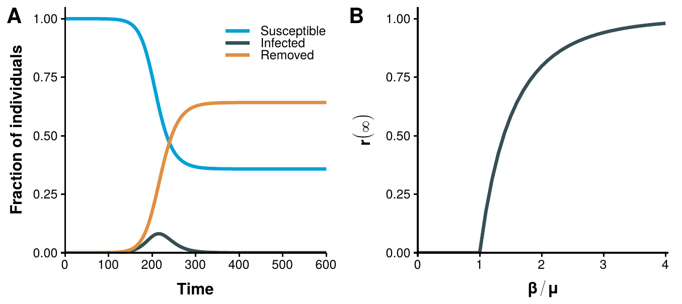
Figure 3.1: Basic results of the homogeneous mixing model. In panel A the evolution of the set of equations (3.9) as a function of time with \(\beta=0.16\) and \(\mu=0.10\) is shown. It is possible to reach a disease free state with a fraction of susceptible individuals larger than 0. In panel B the total fraction of recovered individuals in equilibrium conditions as a function of \(\beta/\mu\) is shown. For simplicity the frequency dependent approach has been used so that the threshold is 1.

At this point a clarification might be in order. During the introduction we said that Hamer had already showed in 1906 that it was possible for an epidemic to end despite the existence of large number of susceptible persons in the population. However, the difference resides in that Hamer proposal was based on data about measles, while this model is formulated without any specific disease in mind. Indeed, although clearly influenced by Hamer’s and Ross’ works, one of the great achievements of Kermack and McKendrick was to establish a formulation based only on mechanistic principles, regardless of the specific properties of the disease. Nonetheless, the most important result of this model has not been discussed yet, the epidemic threshold.

Suppose that in a completely susceptible population we introduce a tiny amount of infected individuals so that \(s(t=0) \equiv s_0 = 1 - \epsilon\) and \(i(t=0) \equiv i_0 = \epsilon\) with \(\epsilon\rightarrow 0\). If we linearize equation (3.10) around this point, we have

\[\begin{equation} \frac{\text{d}i(t)}{\text{d}t} \approx \beta N i_0 s_0 - \mu i_0\,, \tag{3.12} \end{equation}\]

which only grows if \(\beta N - \mu > 0\). Hence, there exists a minimum susceptible population at the initial state below which an epidemic cannot take place, the epidemic threshold:

\[\begin{equation} N_c > \frac{\mu}{\beta}\,. \tag{3.13} \end{equation}\]

Note that the formulation of this threshold can vary slightly according to the characteristics of the model. For instance, in the frequency dependent approach, equation (3.11), the epidemic threshold is defined by

\[\begin{equation} \frac{\beta}{\mu} > 1\,, \tag{3.14} \end{equation}\]

which is independent of \(N\). The existence of this threshold is numerically demonstrated in figure 3.1B, where the final fraction of recovered individuals as a function of the ratio \(\beta/\mu\) is shown. Regardless of the specific shape of the condition, the message is that it is possible to explain why an epidemic might not spread in a population of fully susceptible individuals. Moreover, it also provides a mechanism to fight diseases before they spread. Indeed, in equation (3.13) we have simply considered that \(S_0 = N\), but if we were able to immunize a fraction of the population so that \(S_0 < \mu/\beta\) then the epidemic could not take place. In other words, we would have conferred the population the herd immunity discussed in the beginning of the chapter.

3.1.1 Introducing the age compartment

Since the establishment of epidemiology as a science, a lot of attention has been devoted to the study of measles as its recurring patterns puzzled physicians and mathematicians alike. The distinguishing characteristic of measles epidemics is that they had a very regular temporal pattern with periodic outbreaks of the disease, as shown in figure 3.2. As this disease affects specially the children and also conveys permanent immunity to those who have suffered it, analyzing the time evolution over large time-scales to obtain the patterns required the inclusion of age in the models. Nevertheless, with the basic model that we have analyzed we can already propose a plausible explanation for this behavior. Indeed, we know that if the amount of susceptibles in the population is below a given threshold, the epidemic cannot take place. Thus, it seems reasonable to think that once the epidemic fades-out, there is a period in which there are not enough susceptibles for it to appear again. Yet, when new children are born, the amount of susceptibles will increase, possibly going above the threshold and therefore allowing a new outbreak.

A similar explanation was already proposed by Soper in 1929 [164], although it only matched the observations qualitatively, not quantitatively. It was Barlett who, in 1957, finally provided a quantitative explanation of the phenomenon [165]. Besides the details that we have already discussed, in his proposal he added a new factor that we have not mentioned yet. He proposed that the problem of previous models was that they were deterministic, an approximation that is only valid in very large populations. However, it was observed that the periodicity of measles not only depended on the size of the city, but it was specially so in small towns. In physical terms, we would say that there were finite size effects, tearing down assumption 6 (see section 3.1). Thus, he proposed to use a stochastic model for which he could not obtain a closed form solution, so he had to resort to an “electronic computer”. Nowadays the use of stochastic computational simulations are much more common than the deterministic approach. The reasons why this approach is more favorable are out of the scope of this thesis (see, for instance [140], [166]–[168] for a discussion) but we will leverage this opportunity to say that in the following sections we will mostly work with stochastic simulations, rather than deterministic approaches. Before concluding the discussion about Barlett’s paper, we find worth highlighting that it was presented during a meeting of the Royal Statistical Society, in 1956, after which a discussion followed. In said discussion, Norman T. J. Bailey said “One of the signs of the times is the use of an electronic computer to handle the Monte Carlo experiments. Provided they are not made an excuse for avoiding difficult mathematics, I think there is a great scope for such computers in biometrical work”. And indeed there was, as 25 years later Mr. Bailey was appointed Professor of Medical Informatics [169].

Figure 3.2: Measles epidemics in New York from 1906 to 1948. This figure represents the number of reported cases of measles in the city of New York from 1906 to 1948 with a biweekly resolution. There are some gaps due to missing reports. Data obtained from [170].

Returning to our discussion, it is not surprising, then, that McKendrick already introduced age in his models in 1926 [171], one year before the publication of the full model that we have already explored. However, to introduce age we will use a slightly more modern formulation that will simplify the analysis. In particular, we need to revisit assumption 4, i.e., individuals are only distinguishable by their health status.

Let us state that individuals can now be identified both by their health status and their age. Hence, we have to add more compartments to the model, one for each age group and health status combination. In other words, rather than having three compartments, \(S,I,R\), we now have 3 times the number of age brackets considered, i.e. \(S_a, I_a, R_a\) being \(a\) the age bracket the individuals belong to (see 2.6 for the definition of age bracket). Moreover, we will suppose that the disease dynamics is much faster than the demographic evolution of the population. The only thing left is to decide how to go from one compartment to another:

• For the rate of infectivity, we will define an auxiliary expression that will facilitate the discussion. By inspection of equation (3.9), we can define the force of infection [163] as

\[\begin{equation} \lambda(t) \equiv \phi(\tau) I(t) = \beta I(t)\,, \tag{3.15} \end{equation}\]

which does not depend on any characteristic of the individual. Hence, we can simply incorporate age by modifying the force of infection so that

\[\begin{equation} \lambda(t,a) = \sum_{a'} \phi(\tau,a,a') I_{a'}(t)\,. \tag{3.16} \end{equation}\]

This way, both the age of the individual that is getting infected (\(a\)) and the age of all other individuals (\(\sum_{a'}\)) are taken into account. Furthermore, we can separate \(\phi(\tau,a,a')\) into two components: one accounting for the rate of contacts between individuals of age \(a\) and \(a'\) and another one accounting for the likelihood that such contacts lead to an infection. Hence,

\[\begin{equation} \phi(\tau,a,a') \equiv C(a,a') \beta(a,a')\,. \tag{3.17} \end{equation}\]

Recalling section 2.6, the term \(C(a,a')\) can be obtained from the contact surveys that we have already studied. On the other hand, we will suppose that the likelihood of infection is independent of the age so that \(\beta(a,a') = \beta\).

• For the rate of recovery, we will assume that it is independent of the age of the individual, i.e. \(\mu(a) = \mu\).

Under these assumptions, the homogeneous mixing model with age dependent contacts reads \[\begin{equation} \left\{\begin{array}{l} \frac{\text{d}S_a(t)}{\text{d}t} = - \sum_{a'}\beta C(a,a') I_{a'}(t) S_a(t) \\ \frac{\text{d}I_a(t)}{\text{d}t} = \sum_{a'}\beta C(a,a') I_{a'}(t) S_a(t) - \mu I_a(t) \\ \frac{\text{d}R_a(t)}{\text{d}t} = \mu I_a(t) \end{array}\right. \tag{3.18} \end{equation}\]

Despite its simplicity, this model is still widely used today, specially in the context of metapopulations⁹ [132]. Even more, as in all compartmental models, it is straightforward to extend it to include more complex dynamics. For instance, we can add the exposed state so that individuals that get infected remain in a latent state for a certain amount of time before showing symptoms and being able to infect others. This model, known as the SEIR model, can be used to describe influenza dynamics [173]

\[\begin{equation} \left\{\begin{array}{l} \frac{\text{d}S_a(t)}{\text{d}t} = - \sum_{a'}\beta C(a,a') I_{a'}(t) S_a(t) \\ \frac{\text{d}E_a(t)}{\text{d}t} = \sum_{a'}\beta C(a,a') I_{a'}(t) S_a(t) - \sigma E_a(t)\\ \frac{\text{d}I_a(t)}{\text{d}t} = \sigma E_a(t) - \mu I_a(t) \\ \frac{\text{d}R_a(t)}{\text{d}t} = \mu I_a(t) \end{array}\right. \,. \tag{3.19} \end{equation}\]

The new parameter, \(\sigma\), accounts for the rate at which an individual from the latent state goes to the infectious state, in a similar fashion as \(\mu\) does for the transition from \(I\) to \(R\). This model will be the focus of the last part of this section.

3.1.2 Changing demographics

I call myself a Social Atom - a small speck on the surface of society.
“Memoirs of a social atom”, William E. Adams

As we discussed earlier, for a long period of time the developments in mathematical epidemiology were disconnected from data, at least until Anderson and May arrived to the field in the late 1980s. It is not so surprising, then, that even though age was incorporated into models since the beginning of the discipline, we had to wait until the late 1990s to get experimental data of age mixing patterns.

The first attempt to quantify the mixing behavior responsible for infections transmitted by respiratory droplets or close contact (which are the ones best suited to be studied with homogeneous mixing models) was the pioneering work by Edmunds et al. in 1997 [174]. Their results, however, can hardly be extrapolated as they only analyzed a population consisting of 62 individuals coming from two British universities. The first large-scale experiment to measure these patterns was conducted by Mossong et al. in 2008 [131]. In their study, they measured the age-dependent contact rates in eight European countries (Belgium, Finland, Germany, Great Britain, Italy, Luxembourg, Netherlands and Poland), as part of the European project Polymod, using contact diaries. In the next years other authors followed the route opened by Mossong et al. and measured the age-dependent social contacts of countries such as China [175], France [176], Japan [177], Kenya [178], Russia [179], Uganda [180] or Zimbabwe [181], as well as the Special Administrative Region of Hong Kong [182], greatly expanding the available empirical data.

These experiments provide us with the key ingredient required for the introduction of age compartments into the models, the age contact matrix, \(C\). There are, however, a couple of ways of defining this matrix that are equivalent under certain transformations. We define the matrix in extensive scale, \(C\), as the one in which each element \(C_{i,j}\) contains the total number of contacts between two age groups \(i\) and \(j\). It is trivial to see that given this definition there must be reciprocity in the system, i.e.,

\[\begin{equation} C_{i,j} = C_{j,i}\,. \tag{3.20} \end{equation}\]

A similar definition can be obtained if instead of accounting for all the contacts between two groups we want to capture the average number of contacts that a single individual of group \(i\) will have with individuals in group \(j\):

\[\begin{equation} M_{i,j} = \frac{C_{i,j}}{N_i}\,, \tag{3.21} \end{equation}\]

where \(N_i\) is the number of individuals in group \(i\). We call the matrix in this form the intensive scale. This is the usual format in which this matrix is given. In this case, reciprocity is fulfilled if

\[\begin{equation} M_{i,j} N_i = M_{j,i} N_j\,. \tag{3.22} \end{equation}\]

This last expression rises an interesting question. The reciprocity relation depends on the population in each age bracket, \(N_i\). Thus, if the matrix \(M\) was measured in year \(y\), we have that \(M_{i,j}(y) N_i(y) = M_{j,i}(y) N_j(y)\). However, if we want to use this matrix in a different year, that is, with a different demographic structure due to the inherent evolution of the population, reciprocity will no longer be fulfilled, i.e.

\[\begin{equation} M_{i,j}(y) N_i(y') \neq M_{j,i}(y) N_j(y')\,, \tag{3.23} \end{equation}\]

unless the population has not changed. This is a major problem because there are diseases whose temporal dynamics are comparable to the ones of the demographic evolution. For instance, Tuberculosis is a disease in which age is particularly important and the incubation period ranges from 1 to 30 years [183]. Hence, to properly forecast the evolution of Tuberculosis in a population it is strictly necessary to project somehow these age-contact matrices into the future [134]. Even for diseases that have much shorter dynamics, such as influenza, this is a relevant problem because given how costly these experiments are, it is unpractical to repeat them every few years to obtain updated matrices. As a consequence, if we simply want to study the impact of influenza this year, more than 10 years after the work by Massong et al., we need to devise a way to properly update them.

Figure 3.3 exemplifies, for Poland and Zimbabwe, the error we would make if we do not adapt \(M\) and blindly use it with demographic structures that are different than the original. We define the reciprocity error as

\[\begin{equation} E = \frac{\sum_{i,j>i} |C_{i,j}-C_{j,i}|}{0.5\cdot \sum_{i,j} C_{i,j}} = \frac{\sum_{i,j>i} | M_{i,j} N_i - M_{j,i} N_j |}{0.5 \cdot \sum_{i,j} M_{i,j} N_i}\,, \tag{3.24} \end{equation}\]

to quantify the fraction of links that are not reciprocal. The two countries under consideration have very different demographic patterns, both in the past and in the future, and yet we can see that the error is quite large in both of them.

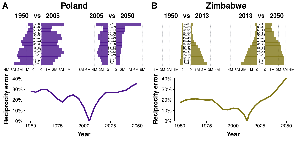
Figure 3.3: Reciprocity error as a function of time in Poland and Zimbabwe. For each country, in the top plots the demographic structures of 1950 and 2050 are compared to the one existing when the contact matrices were measured. In the bottom plot the reciprocity error as a function of time is shown. For the matrix to be correct in different years the error should be 0, but that only happens in the year when the data was collected.

The problem is that both \(C_{i,j}\) and \(M_{i,j}\) implicitly contain information about the demographic structure of the population at the time they were measured. To solve this problem, we define the intrinsic connectivity matrix as

\[\begin{equation} \Gamma_{i,j} = M_{i,j} \frac{N}{N_j}\,. \tag{3.25} \end{equation}\]

This matrix corresponds, except for a global factor, to the contact pattern in a “rectangular” demography (a population structure where all age groups have the same density). Hence, it does not have any information about the demographic structure of the population.

In figure 3.4A we show the instrinsic connectivity matrices for each of the 16 regions enumerated previously. Interestingly, the contact patterns are quite different from region to region. To facilitate the comparison, in figure 3.4B we plot the fraction of connectivity that corresponds to young individuals (less than 20 years old) as a function of the assortativity of each matrix as defined by Newman [73] (this quantity is an adaptation of the Pearson correlation coefficient so that it is equal to 1 if individuals tend to contact those who are like them, -1 in the opposite case and 0 if the pattern is completely uncorrelated). We can see that regions with similar demographic structures and culture tend to cluster together, although it is not possible to disentangle which is the precise cause leading to one pattern or the other.

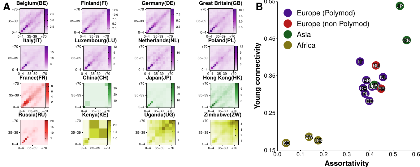
Figure 3.4: Age contact matrices from 16 regions. A) Intrinsic connectivity matrix, \(\Gamma_{i,j}\), of each region. There is not a standard definition of age brackets and thus each study had its own definition. For comparison purposes, we have adapted the data to 15 age brackets: \([0,5),[5,10),\ldots,[65,70),+70\). B) Proportion of connectivity corresponding to individuals younger than 20 versus the assortativity coefficient of each matrix.

With this matrix we can now easily compute \(M\) at any other time, as long as we know the demographic structure of the population at that time:

\[\begin{equation} M_{i,j} (y') = \Gamma_{i,j} \frac{N_j(y')}{N(y')} = M_{i,j}(y) \frac{N(y)N_j(y')}{N_j(y)N(y')}\,. \tag{3.26} \end{equation}\]

In our case, we will obtain this data from the UN population division database, which contains information of both the past demographic structures and their projections to 2050 for the whole world [184].

We conclude this section addressing how this correction impacts disease modeling. To this end, we simulate the spreading of an influenza-like disease both with and without corrections on the matrix. We choose influenza because it is a short-cycle disease so that we can assume that the population structure is constant during each simulated outbreak. Besides, it can be effectively modeled using the SEIR model presented in 3.1.1.

To parameterize the model we use the values of an influenza outbreak that took place in Belgium in the season 2008/2009 [132]. Thus, individuals can catch the disease with transmissibility rate \(\beta\) per-contact with an infectious individual. The value of \(\beta\) is determined in each simulation so that the basic reproductive number is equal to \(2.12\) using the next generation approach (this procedure will be explained in more detail in section 3.2) [132], [185]. Once infected, individuals remain on a latency state for \(\sigma^{-1} = 1.1\) days on average. Then, they become infectious for \(\mu^{-1} = 3\) days on average, period when they can transmit the infection to susceptible individuals. After that, they recover and become immune to the disease. We use a discrete and stochastic model with the population divided into 15 age classes, whose mixing is given by the age contact matrix \(M\). To sum up:

• The probability of an individual belonging to age group \(i\) to get infected is

\[\begin{equation} p_{S\rightarrow E} = \beta \sum_j \frac{M_{i,j}}{N_j} I_j\,. \tag{3.27} \end{equation}\]

• Once in the latent state, the probability of entering the infected state is

\[\begin{equation} p_{E\rightarrow I} = \sigma\,. \tag{3.28} \end{equation}\]

• Finally, an infected individual will recover with probability

\[\begin{equation} p_{I\rightarrow R} = \mu\,. \tag{3.29} \end{equation}\]

Under these conditions, we compute the predicted size of the epidemic, i.e., \(R(t\rightarrow \infty)\), in years 2000 and 2050. In figure 3.5 we present the results. In particular, in A we show the difference between the predicted size of the epidemic in 2050 versus the one in 2000 using the same \(M\) matrix in both years. In almost all countries the final size of the epidemic is smaller in 2050, except for China and the African countries in which it increases. However, in B we repeat the analysis but using the adapted values of \(M(y')\) obtained using (3.26). In this case, in general, the situation is reversed. Most countries have larger epidemics, except for the African ones. Even more, in countries such as China and Japan the difference is quite large, close to 20%.

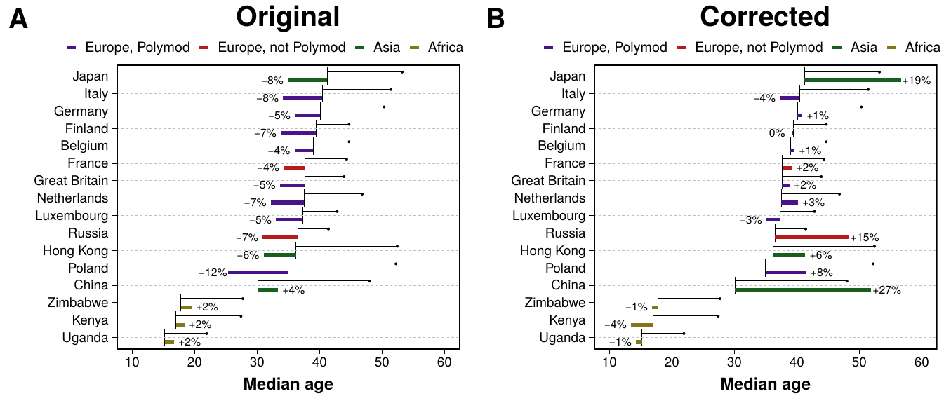
Figure 3.5: Predictions of influenza incidence in 2050 with demographic corrections. In both plots the black horizontal line starts at the median age of each region in the year 2000 and ends with a bullet point with the predicted value in 2050. Color bars denote the relative variation of incidence over the same period. In A the predictions are computed using the original contact matrices collected from the surveys. In B the proposed demographic corrections are applied to the matrices.

Summarizing, to create more realistic models we need to incorporate empirically measured data. However, blindly using data without thinking whether it can be applied to the specific system we are studying is not adequate. In the particular case of social mixing matrices, we have seen that even if we keep studying the same country, just moving a few years away from the moment in which the experiment took place dramatically affects the reciprocity of the contacts. This, in turn, leads to important differences in the global incidence for influenza-like diseases, as we have shown in our analysis of the SEIR model. Even more, since there are different intrinsic connectivity patterns across countries, it is possible that there exists a time evolution of this quantity. Indeed, if we believe that the intrinsic pattern is a consequence of the culture of the country, it seems logical to think that an evolving culture will also have evolving intrinsic connectivity patterns. Although predicting how society will change in the future is currently impossible, this should be taken into account as a limitation in any forecast for which heterogeneity in social mixing is a key element.

3.2 The basic reproduction number

One of the cornerstones of modern epidemiology is the basic reproduction number, \(R_0\), defined as the expected number of individuals infected by a single infected person during her entire infectious period in a population which is entirely susceptible. From this definition, it is clear that if \(R_0<1\), then, each infected individual will produce, on average, less than one infection. Therefore, the disease will not be able to be sustained in the population. Conversely, if \(R_0>1\) the disease will be able to propagate to a macroscopic fraction of the population. Hence, this simple dimensionless quantity is informing us of three key aspects of a disease: (1) whether the disease will be able to invade the population, at least initially; (2) a way to determine which control measures, and at what magnitude, would be the most effective, i.e., which ones will reduce \(R_0\) below 1; (3) to gauge the risk of an epidemic in emerging infectious diseases [186].

Interestingly, despite its importance, this quantity was not originated in epidemiology. The concept of \(R_0\), and its notation, was formalized by Dublin and Lotka, in 1925, in the context of demography¹⁰ [188]. The similitude of the concept in both fields is obvious, in one it measures the number of new infections per infected while in the other the number of births per female. Yet, in epidemiology the concept was mostly unknown until Anderson and May popularized it 60 years later in the Dahlem conference [189] (see [190] for a nice historical discussion on why it took so long for this concept to mature in epidemiology).

It might be enlightening to introduce the mathematical definition from the point of view of demography. Consider a large population. Let \(F_d(a)\) be the survival function, i.e., the probability for a new-born individual to survive at least to age \(a\), and let \(b(a)\) denote the average number of offspring that an individual will produce per unit of time at age \(a\). The function \(n(a) \equiv b(a) F_d(a)\) is called the reproduction function. Hence, the expected future offspring of a new-born individual, \(R_0\), is [191]

\[\begin{equation} R^{demo}_0 \equiv \int_0^\infty n(a) \text{d} a = \int_0^\infty b(a) F_d(a) \text{d}a\,. \tag{3.30} \end{equation}\]

The translation of this definition to epidemiology is straightforward. First, note that the reproduction function at age \(a\) is equivalent to the expected infectivity of an individual who was infected \(\tau\) units of time ago, \(A(\tau)\) (see equation (3.4)). There is, however, one crucial difference. While in demography it is possible to “create” new individuals regardless of the size of the rest of the population, in epidemiology the creation of new individuals depends both on the infectivity and on the amount of susceptible individuals in the population. Hence,

\[\begin{equation} R_0(\eta) \equiv \int_\Omega S(\xi) \int_0^\infty A(\tau,\xi,\eta)\text{d}\tau \text{d}\xi\,. \tag{3.31} \end{equation}\]

This rather cryptic expression is the most general definition of this quantity [192], although we will see in a moment simpler ones. The expression should be read as follows: the value of \(R_0\) for individuals in an infectious state \(\eta\) is equal to the sum of all individuals in a susceptible state characterized by \(\xi\), of size \(\Omega\), times the infectivity of individuals in said state \(\eta\) who where infected \(\tau\) steps ago and can infect individuals in state \(\xi\).

In the particular case of the SIR model under the density dependent approach, equation (3.9), the basic reproduction number is simply

\[\begin{equation} \begin{split} R_0 & = S_0 \int_0^\infty A(\tau) \text{d}\tau = S_0 \int_0^\infty \beta e^{-\mu \tau} \text{d}\tau \\ & = \frac{\beta S_0}{\mu}\,, \end{split} \tag{3.32} \end{equation}\]

where \(S_0\) is the number of susceptible individuals at the beginning of the infection, which in the absence of immunized individuals is equal to \(N\). Recall that the linear stability analysis of the SIR model (3.12) yields,

\[\begin{equation} i(t) = i_0 e^{\beta N- \mu}\,, \tag{3.33} \end{equation}\]

which only grows if \(\beta N > \mu\). In other words, \(R_0\) defines precisely the epidemic threshold that we found in the previous section, i.e.,

\[\begin{equation} R_0 = \frac{\beta N}{\mu} > 1\,, \tag{3.34} \end{equation}\]

as heuristically discussed at the beginning of this section. In the frequency dependent approach, which is more common in the network science literature as we shall see in 3.3, the basic reproduction number¹¹ is

\[\begin{equation} R_0 = \frac{\beta}{\mu} > 1\,. \tag{3.35} \end{equation}\]

To obtain an explicit expression for \(R_0\) with more complex compartmental models, an alternative approach to linear stability analysis is the next generation matrix as proposed by Diekmann in 1990 [192] and further elaborated by van den Driessche and Watmough in 2002 [185]. Briefly, the idea is to study the stability of the disease free state, \(x_0\). To do so, we restrict the model to those compartments with infected individuals and separate the evolution due to new individuals getting infected, \(\mathcal{F}\), and the transitions resulting for any other reason,

\[\begin{equation} \frac{\text{d}x_i(t)}{\text{d}t} = \mathcal{F}_i(x) - \mathcal{V}_i(x)\,, \tag{3.36} \end{equation}\]

where \(x = (x_1,\ldots,x_m)\) denotes the \(m\) infected states in the model. If we now define

\[\begin{equation} F = \left[\frac{\partial \mathcal{F}_i(x_0)}{\partial x_j}\right] \text{~~and~~} V = \left[\frac{\partial \mathcal{V}_i(x_0)}{\partial x_j}\right]\,, \tag{3.37} \end{equation}\]

the next generation matrix is \(FV^{-1}\) and the basic reproductive number can be obtained as

\[\begin{equation} R_0 = \rho(FV^{-1})\, \tag{3.38} \end{equation}\]

where \(\rho\) denotes the spectral radius [193]. In particular, for the model considered in section 3.1.2, the next generation matrix reads

\[\begin{equation} K_{i,j} = \frac{\beta}{\mu} \frac{M_{i,j}}{N_j}\,. \tag{3.39} \end{equation}\]

This expression can be used to ensure that, regardless of the values of \(M_{i,j}\) and \(N_j\), the starting point of the dynamics is the same. For this reason, when we wanted to address the differences in incidence consequence of the changing demographics, we fitted \(\beta\) so that the spectral radius of (3.39) was always \(R_0 = 2.12\).

It is worth pointing out that \(R_0\) clearly depends on the model we choose for the dynamics. As a consequence, even though its epidemiological definition is completely independent from models (number of secondary infections per infected individual in a fully susceptible population), its mathematical formulation is not univocal. Ideally, if in a disease outbreak we knew who infected whom, we would be able to obtain the exact value of \(R_0\). In reality, however, this information is seldom available. Hence, to compute it, one often relies on aggregated quantities, such as \(\beta\) and \(\mu\) in equation (3.35). The problem is that if we assume that a disease can be modeled within a specific framework, we cannot directly compare the value obtained for \(R_0\) with the ones measured for other diseases unless the exact same model has been used to obtain it. This is one of the observations that will motivate our work, which we will describe in section 3.2.3.

3.2.1 Measuring \(\mathbf{R_0}\)

Measuring \(R_0\) is not an easy task, specially in the case of emergent diseases for which fast forecasts are required. An accurate estimation of its value is crucial to planning for the control of an infection, but usually the only available information about the transmissibility of a new infectious disease is restricted to the daily count of new cases. Fortunately, it is possible, under certain conditions, to obtain an expression for \(R_0\) as a function of that data.

Following [194], we will assume that in the beginning of a disease outbreak the growth of the number of infected individuals is exponential. Hence, the number of new infected individuals at time \(t\) will be equal to the number of new infected individuals \(\tau\) time units ago, multiplied by the exponential growth,

\[\begin{equation} \frac{\text{d}S(t)}{\text{d}t} = \frac{\text{d}S(t-\tau)}{\text{d}t} e^{r\tau}\, \tag{3.40} \end{equation}\]

where \(r\) denotes the growth rate. Inserting this expression in (3.1) with \(t\rightarrow 0\),

\[\begin{equation} \frac{\text{d}S(t)}{\text{d}t} = S(t=0) \int_0^\infty A(\tau) \frac{\text{d}S(t)}{\text{d}t} e^{-r\tau} \text{d}\tau \Rightarrow 1 = S_0 \int_0^\infty A(\tau) e^{-r\tau} \text{d}\tau \tag{3.41} \end{equation}\]

At this point it might be enlightening to return once again to the demographic simile. In equation (3.30) we saw that the total number of offspring of a person could be obtained integrating \(n(a)\) (rate of reproduction at age \(a\)) over the whole lifespan of the individual. Thus, we can define the distribution of the age a person has when she has a child as

\[\begin{equation} g'(a) = \frac{n(a)}{\int_0^\infty n(a) \text{d} a } = \frac{n(a)}{R_0^{demo}}\,. \tag{3.42} \end{equation}\]

If we take the “age” of an infection to be the time since the infection, we can define an analogous quantity in epidemiology,

\[\begin{equation} g(\tau) = \frac{S_0 A(\tau)}{R_0}\,, \tag{3.43} \end{equation}\]

called generation interval distribution. In this case this distribution is the probability distribution function for the time from infection of an individual to the infection of a secondary case by that individual. Going back to (3.41) we now have

\[\begin{equation} \frac{1}{R_0} = \int_0^\infty g(\tau) e^{-r\tau} \text{d}\tau\,. \tag{3.44} \end{equation}\]

According to this last expression, the shape of the generation interval distribution determines the relation between the basic reproduction number \(R_0\) and the growth rate \(r\). In all the models explored so far, we assumed that both the rate of infection \(\beta\) and the rate of leaving the infectious stage \(\mu\) were constant. Hence, it follows that the duration of a generation interval is specified as an exponential distribution with mean \(Tg = 1/\mu\). Under these assumptions the basic reproduction number is then

\[\begin{equation} \begin{split} R_0 & = \left( \int_0^\infty \mu e^{-\mu\tau} e^{-r\tau} \text{d} \tau\right)^{-1} = \left( \frac{\mu}{r+\mu} \right)^{-1} \\ & = 1 + rTg \,. \end{split} \tag{3.45} \end{equation}\]

This relation between the growth rate and the generation time was already proposed by Dietz in 1976 [195], although only in the specific case of the SIR model. Equation (3.44), however, allows for the calculation of \(R_0\) in more complex scenarios, such as non constant \(\mu\) [194]. Despite its limitations, this expression is widely used in the literature due to its simplicity. Indeed, \(Tg\) is often considered to be simply the inverse of the recovery rate, which is relatively easy to measure. Thus, \(r\) can be obtained by fitting a straight line to the cumulative number of infections as a function of time, see (3.40).

There are, however, several problems with this procedure. First, we stated that the exponential growth is valid during the early phase of an outbreak, but there is no way to know how long is that in general. As a consequence, when one fits a straight line to the data, some heuristics have to be used to determine which points to use. Even more, if the dynamics is really fast there might be just a few valid points. Given the stochasticity of the process, this might lead to poor estimates of the growth rate.

Besides, there are some caveats on the exponential growth assumption. For instance, it has been observed that for some diseases such as AIDS/HIV the early growth is sub-exponential [196]. Likelihood based methods in which the early exponential growth is not needed were thus proposed [197], [198]. But even for diseases in which it might be a good approximation, there is the problem of susceptible depletion. Indeed, if the population is infinite, each infected individual will be always able to reach an infinite amount of susceptibles. But this is not true in real situations, forbidding the exponential growth to be sustained for too long. Hence, methods that account for this depletion during the initial phase had also to be developed [199], [200].

It should be clear by now that despite the widespread use of this parameter, it is far from being perfectly understood, specially in the presence of real world data. Yet, we can go one step further and generalize the definition of \(R_0\) to the effective reproduction number, \(R(t)\).

3.2.2 The effective reproduction number

The effective reproduction number, \(R(t)\), is defined as the average number of secondary cases generated by an infectious individual at time \(t\). Hence, we are relaxing the hypothesis of a fully susceptible population that we gave at the beginning of section 3.2.

This parameter is obviously better suited for studying the impact of protection measures taken after the detection of an epidemic, as it can be defined at any time. If \(R(t)<1\), it seems reasonable to say that the epidemic is in decline and may be regarded as being under control at time \(t\). Furthermore, in section 3.1.1 we saw that diseases such as measles have periodic outbreaks and also convey immunity to those who have suffered it. Thus, when a new outbreak starts the population is not completely susceptible, invalidating one of the conditions in the definition of \(R_0\) [201].

To provide a mathematical definition of \(R(t)\) [202], we can revisit equation (3.32) and define

\[\begin{equation} R(t) = S(t) \int_0^\infty A(\tau)\text{d}\tau\,, \tag{3.46} \end{equation}\]

which leads to

\[\begin{equation} R(t) = \frac{S(t)}{S_0} R_0\,. \tag{3.47} \end{equation}\]

According to this expression, in a closed population, the value of \(R(t)\) should monotonically decrease. As expected, this has been observed in computational simulations [201], even in the case of sub-exponential growth [203]. However, this is not always the case if one tries to obtain \(R(t)\) from real data [204]. In particular, Walling and Teunis studied the severe acute respiratory syndrome (SARS) epidemic from 2003 and observed several local maxima in the evolution of the effective reproduction number, which they attributed to “super-spread events” in which certain individuals infected unusually large numbers of secondary cases [205]. This was also found in other diseases, signaling that the whole complexity of real systems cannot be completely captured with simple homogeneous models [206]. For this reason, the next section will be devoted to our contribution in the study of the effect that more heterogeneous population distributions have on the reproduction numbers.

3.2.3 Measurability of the epidemic reproduction number

Of course, there had been plenty of diseases, long before humans had been around. But humans had definitely created Pestilence. They had a genius for crowding together, for poking around in jungles, for setting the midden so handily next to the well. Pestilence was, therefore, part human, with all that this entailed.
“Thief of time”, Terry Pratchett

The fundamental role that households play in the spreading of epidemics has been acknowledged for a long time. Early estimations of influenza spreading already showed that the probability of getting infected from someone living in your household or someone from the community were quite different. Even more, it was shown that children were twice more likely to get the infection from the community than adults, signaling that the places that children visit and the own heterogeneity of household members are fundamental in the disease dynamics [207]. In a more recent study, data from a real epidemic in a small semi-rural community was analyzed, with schools added explicitly into the picture. As expected, it was observed that their role is key in the spreading of the disease. But, even more interesting, the authors calculated a reproduction number for each population structure and found it to be smaller or of the order of 1, meaning that for an outbreak to be sustained a complex interplay between those structures must take place [208].

In order to introduce the concept of households into the models analyzed so far, we need to revisit once again the assumption of full homogeneity. Most theoretical approaches in this line, since the seminal work of Ball et al. in 1997 [209], have focused on what is known as models with two levels of mixing. In these models, a local homogeneous mixing in small environments (such as households) is set over a background homogeneous mixing of the whole population. This can be further extended by adding other types of local interactions, such as schools or workplaces. An individual can thus belong at the same time to two or more local groups. For this reason, they are also known as overlapping group models [210]. This allows for the definition of several basic reproduction numbers, one for the community and the rest for local interactions, which in turn can be used to devise efficient vaccination strategies [211], [212]. Other studies have also proposed that the generation time can differ from within households and the community [213].

However, theoretical studies have been mostly focused on the early phase of the epidemics because it is more mathematically tractable. Yet, we have seen in the previous section that \(R(t)\) can provide very important insights to understand the dynamics of real diseases. For this reason, statistical methods have been developed to analyze \(R(t)\) [214], [215]. Unfortunately, for these methods, disentangling the role that each structure of the system plays is challenging due to the lack of microscale data on human contact patterns for large populations. Note also that due to the typically small size of households, stochastic effects are highly important.

In this work our objective is to shed some light into the mechanisms behind disease dynamics in heterogeneous populations. To do so, we study the evolution of \(R(t)\) and \(Tg\) with data-driven stochastic micro-simulations of an influenza-like outbreak on a highly detailed synthetic population. The term “micro” refers to the fact that we will keep track of each individual in the population, allowing us to reconstruct the entire transmission chain. The great advantage of this method is that it allows for the computation of \(R(t)\) from its own epidemiological definition, without requiring any mathematical approximation.

Our synthetic population is composed by 500,000 agents, representing a subset of the Italian population. This population model, developed by Fumanelli et al. [216], divides the system into the four settings where influenza transmission occurs, namely households, schools, workplaces and the general community [217]. Henceforth we will refer to these settings as layers for the similarity of this construction to the multilayer networks we saw in section 2.1.3¹²; a visualization of the model is shown in 3.6A. The household layer is composed by \(n_H\) disconnected components, each one representing one household. The amount of individuals inside each household is determined by sampling from the actual Italian household size distribution, as well as their age. Then, by sampling from the multinomial distribution of schooling and employment rates by age, each individual might be also assigned to a school or workplace. Both the number and size of workplaces and schools is also sampled from the actual Italian distribution. As in the household layer, each of the \(n_S\) schools and \(n_W\) workplaces are disconnected from the rest in their respective layers. Lastly, all individuals are allowed to interact with each other in the community layer, encapsulating the background global interaction. To highlight the heterogeneity of the system, in figure 3.6B the size distribution of the places each individual belongs to is shown. Note that while most households contain 2-3 individuals and most schools are close to 1,000 students, workplaces cover a much wider range of sizes.

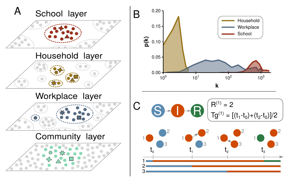
Figure 3.6: Model structure of a synthetic population organized in schools, households and workplaces. A) Visualization of the overlapping system, with individuals being able to interact locally in multiple contexts. B) Distribution of the structure size each individual belongs to. C) Illustration of the transmission process with an example of how to calculate the reproduction number and generation interval.

The influenza-like transmission dynamics are defined through the susceptible, infected, removed (SIR) compartmental model that we have been analyzing under diverse assumptions. We simulate the transmission dynamics using a stochastic process for each individual, keeping track of where she contracted the disease, who is in contact with and so on. In order to resemble an influenza-like disease, the local spreading power in each layer is calibrated in such a way that the fraction of cases in the four layers is in agreement with literature values (namely, 30% of all influenza infections are linked to transmission occurring in the household setting, 18% in schools, 19% in workplaces and 33% in the community [218]). Hence, the probability that individual \(j\) infects \(i\) in layer \(l\) is

\[\begin{equation} \beta = w_l\,, \tag{3.48} \end{equation}\]

as long as \(j\) is infected, \(i\) is susceptible and both belong to the same component in layer \(l\). Moreover, we set the values of \(w_l\) such that the basic reproduction number is \(R_0=1.3\) [219]. Finally, the removal probability, \(\mu\), is set so that the removal time is 3 days [220].

The epidemic starts with a fully susceptible population in which we set just one individual as infected. Thanks to the microscopic detail of the model, we can thus compute the basic reproduction number directly as the number of infections that said first individual produces before recovery. Its counterpart over time, the effective reproduction number, \(R(t)\), is measured using the average number of secondary cases generated by an infectious individual at time \(t\). Similarly, we also define the effective reproduction number in layer \(l\), \(R_l(t)\), as the average number of secondary infections generated by a typical infectious individual in layer \(l\):

\[\begin{equation} R_l(t) = \frac{\sum_{i\in \mathcal{I}(t)} D_l(i)}{|\mathcal{I}(t)|}\,, \tag{3.49} \end{equation}\]

where \(\mathcal{I}(t)\) represents the set of infectious individuals that acquired the infection at time \(t\) and \(D_l(i)\) the number of infections generated by infectious node \(i\) in layer \(l\) with \(l \in L=\{H,S,W,C\}\). With this expression we can obtain the overall reproductive number as

\[\begin{equation} R(t) = \sum_{l\in L} R_l(t)\,. \tag{3.50} \end{equation}\]

The generation time \(Tg\) is defined as the average time interval between the infection time of infectors and their infectees. Hence, analogously to the reproduction number, we define the generation time in layer \(l\) as

\[\begin{equation} {Tg}_l = \frac{\sum_{i\in \mathcal{I}(t)} \sum_{j \in \mathcal{I}'_l(i)} (\tau(j)-t)}{\sum_{i \in \mathcal{I}(t)} D_l(i)}\,, \tag{3.51} \end{equation}\]

where \(\mathcal{I}'_l(i)\) denotes the set of individuals that \(i\) infected in layer \(l\) and \(\tau(j)\) is the time when node \(j\) acquired the infection. Therefore, the overall generation time \(Tg(t)\) reads

\[\begin{equation} Tg(t) = \frac{\sum_{l\in L}\sum_{i \in \mathcal{I}(t)} \sum_{j \in \mathcal{I}'_l(i)} (\tau(j)-t)}{\sum_{l\in L}\sum_{i\in \mathcal{I}(t)} D_l(i)}\,. \tag{3.52} \end{equation}\]

A schematic illustration of the transmission dynamics is shown in figure 3.6C. In that case, individual 1 gets infected at \(t=t_0\), while individuals 2 and 3 are still susceptible. During the course of her disease individual 1 infects individual 2 at \(t=t_1\) and individual 3 at \(t=t_2\) before finally getting recovered at \(t=t_3\). Thus, her reproduction number is equal to 2 and her generation time is \(1.5\), supposing that \(t_{i+1} - t_i = 1\). In fact, in our simulations we will set \(\Delta t = 1\) day. Due to the stochasticity of the process, each realization might result in an outbreak of different length. Hence, the time evolution of each simulation is aligned so that the peak of the epidemic is exactly at \(t=0\). The results for the reproduction number and generation time are shown in figure 3.7.

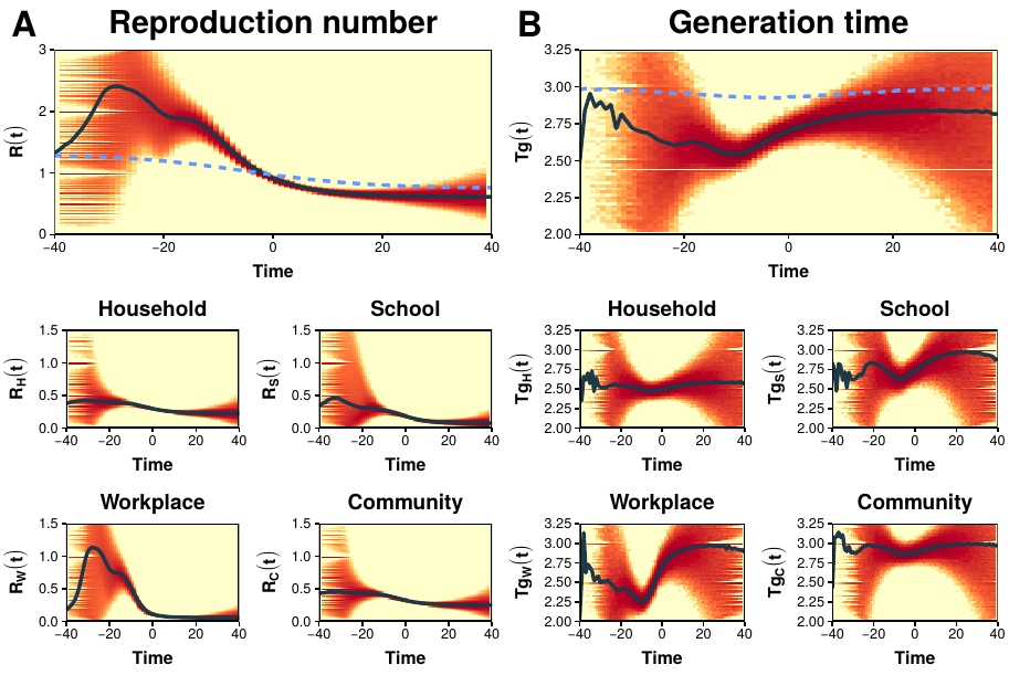
Figure 3.7: Fundamental epidemiological indicators. A) Top: mean \(R(t)\) of data-driven model (solid line) compared to the solution under a completely homogeneous population (dashed line). The colored area shows the density distribution of \(R(t)\) values obtained in single realizations of the model. Bottom: the reproductive number is broken down in the four layers. B) As A but for the generation time. In all cases the simulations have been aligned at the peak of the epidemic.

We find that \(R(t)\) increases over time in the early phase of the epidemic, starting from \(R_0 = 1.3\) to a peak of about \(2.5\) (figure 3.7A). In contrast, in the homogeneous model (dashed line), which lacks the typical structures of human populations, \(R(t)\) is nearly constant in the early epidemic phase and then rapidly declines before the epidemic peak (\(t=0\)), as predicted by the classical theory. The non-constant phase of \(R(t)\) implies that \(R_0\) loses its meaning as a fundamental indicator in favor of \(R(t)\). In figure 3.7B we show an analogous analysis of the measured generation time in the data-driven model. In this case, we find that \(Tg\) is considerably shorter than the infectious period (\(3\) days), with a more marked shortening near the epidemic peak. Once again, in the homogeneous model (dashed line) the behavior predicted by the classical theory is recovered.

A closer look at the transmission process in each layer helps to understand the origin of the deviations from classical theory. Specifically, we see that \(R(t)\) tends to peak in the workplace layer, and to some extent also in the school layer. In the community layer, on the other hand, the behavior is much closer to what is expected in a classical homogeneous population. We also find that \(Tg\) is remarkably shorter in the household layer than in all other layers. This could simply be due to a depletion of susceptibles. To illustrate this, suppose that an infected individual in a household of size 3 infected one of the other two. Then, during the next time step both will compete to infect the last susceptible, something that does not happen in large populations. This would lead to a shorter generation time simply because she is unable to infect other members, even if she is still infected. This evidence calls for considering within household competition effects when analyzing empirical data of the generation time.

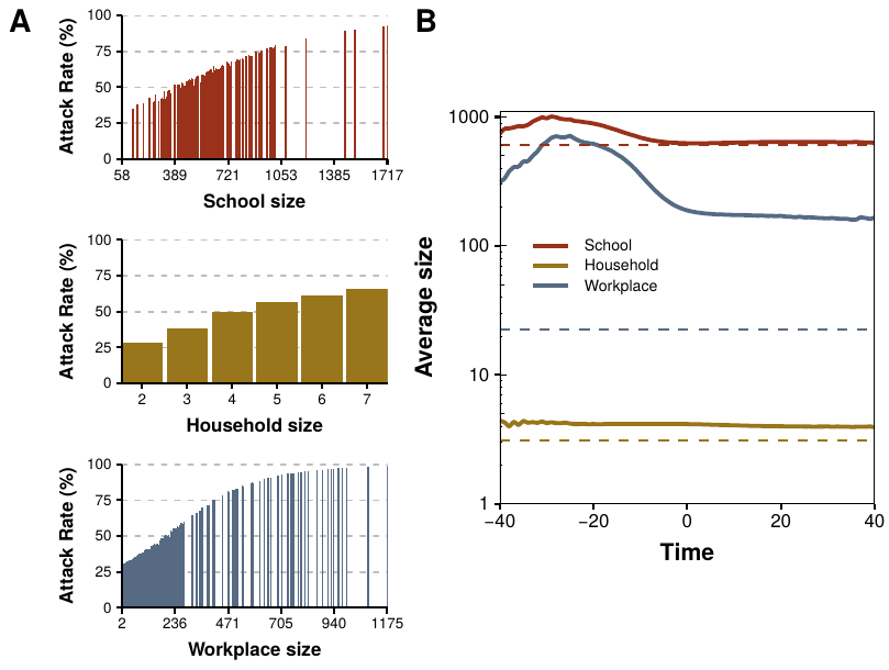
Figure 3.8: Attack rate as a function of site size. A) Fraction of individuals belonging to each place that contracted the disease, not necessarily in said setting. B) Solid line: average size of places in which there is at least one new infection in each time step, broken down in three layers. Dashed line: expected size if there is at least one infection in every place.

To further understand the reasons of the diverse trends observed in each layer, in figure 3.8 we analyze the effect that the size of the components has on the dynamics. In figure 3.8A we study the attack rate (final fraction of removed individuals, i.e., individuals that suffered the infection at some point) as a function of the site size, distinguishing the three layers. The results indicate that the spreading is much more important in large buildings, but we know that they are scarce (see figure 3.6B). Hence, it seems that the initial growth of the epidemic might stop once the big components have been mostly infected. This is corroborated in figure 3.8B, where the average size of buildings with at least one infection is shown. The situation is thus clear. In the classical model not only it is assumed that all population is initially susceptible, but also that it is in contact with the first infected since the beginning. In heterogeneous populations, however, the first infected individual has only a handful of local contacts, diminishing its infectious power. Then, as the epidemic progresses more and more susceptibles enter into play, increasing the amount of individuals that can be infected. Yet, sooner or later the components will run out of susceptibles, even if there is still a large fraction available in the rest of the system. This, in turn, leads to a more abrupt descent than what is expected in the classical approximation.

These results clearly highlight how the heterogeneity of human interactions (i.e., clustering in households, schools and workplaces) alters the standard results of fundamental epidemiological indicators, such as the reproduction number and the generation time. Furthermore, they call into question the measurability of \(R_0\) in realistic populations, as well as its adequacy as an approximate descriptor of the epidemic dynamics. Lastly, our study suggests that epidemic inflection points, often ascribed to behavioral changes or control strategies, could also be explained by the natural contact structure of the population. Hopefully, this analysis will open the path to developing better theoretical frameworks, in which some of the most fundamental assumptions of epidemiology have to be revisited.

3.3 The epidemic threshold fades out

In epidemiology attention has historically been restricted to biological factors. We began this chapter stating that individuals were just indistinguishable particles interacting according to the mass action law. However, throughout the following sections, we have shown that when this oversimplification is relaxed many interesting phenomena arise. In this section we shall go one step further and completely remove what we called assumptions 3 and 4: mass action and indistinguishability. To distinguish individuals, we will assign to each of them an index, \(i\). Then, we will allow individuals to spread the disease only to those with whom they have some kind of contact (e.g. they are friends), which we will encode in links. In other words, we are finally going to introduce networks into the picture.

It is rather difficult to establish the origin of what we may call disease spreading on networks or network epidemiology. Probably, one of the earliest attempts is the work by Cochran, in 1936 [221], in which he studied the propagation of a disease in a small plantation of tomatoes. Although his work might be better described as statistical analysis, the reason to consider it one of the precursors of the spreading on networks is that, as Kermack and McKendrick had done roughly 10 years before, his assumptions were all mechanistic rather than based on the knowledge of the particular problem. This is clearly seen in how he introduced the model: “We suppose that in the first [day] each plant in the field has an equal and independent chance \(p\) of becoming infected, and that in the second [day] a plant which is next to a diseased plant has a probability \(s\) of being infected by it, healthy plants which are not next to a diseased plant remaining healthy”. In modern terminology, the plants were arranged in a lattice structure and could infect their first neighbors with probability \(s\). The assumptions are particularly strong because he knew that the disease was propagated by an insect, but decided to create a very general model.

During the next couple of decades, lattice systems were quite popular in physics, geography and ecology. Then, in the 1960s the interest in studying the spatial spread of epidemics started to grow (see the introduction of [222] for a nice overview) with three main approaches. In the first, the agents that could be infected were set in the center of a certain tessellation of space and could only infect/be infected by their neighbors. This is the closest approach to the modern study of epidemics on networks, but it was not so popular as it was mainly used to study plant systems [223]. The most popular approach was to distribute individuals continuously in space with some chosen density. This led to the study of diffusion processes, focusing on the interplay between velocity and density [224]. The third approach was based on what we briefly defined in section 3.1.1 as metapopulations. Recall that in a metapopulation individuals are arranged in a set of sub-populations. Within each sub-population usually homogeneous mixing is applied and it is also allowed to have individuals migrating from one sub-population to another. Hence, the idea was to simulate the fact that people (or animals) live in a certain place where they can contract the disease, and then travel to a different area and spread it to its inhabitants [168]. Note, however, that in none of these methods we are taking into account any sociological factors of the population.

In the beginning of the 1980s some results pointing into the direction of introducing more complex networks started to appear. In particular, von Bahr and Martin-L"{o}f in 1980 [225] and Grassberger in 1983 [226] (in the context of percolation) showed that the classical SIR model on a homogeneous population could be related to the ER graph model that we saw in section 2.1.2. Indeed, suppose that we have a set of individuals under the homogeneous mixing approach and simulate an epidemic. Next, if an individual \(i\) infects another individual \(j\), we establish a link between them. If the probability of this event is really low, the epidemic will not take place. Conversely, for large probabilities most nodes will be randomly connected. This is precisely how we defined the ER model, with the only difference being that the probability \(p\) of establishing a link will be a function of both the probability of infecting someone, \(\beta\), and that of getting recovered, \(\mu\). Note, however, that they did not implement a disease dynamics on a network, but rather extracted the network from the results of the dynamics.

Roughly at the same time, the gonorrhea rates rose precipitously. To understand the dynamics of this venereal disease, it was recognized that some sort of nonrandom mixing of the population had to be incorporated to the models. The first attempts were based on separating the contact process and the spreading process [227]. Indeed, going back to the definition of the SIR model, we defined the rate of infectivity (3.5) as \(\phi(\tau) = \beta/N\) (under the frequency approach). We can simply define $= c ’ $ where \(c\) is the contact rate between individuals and \(\beta '\) the probability of spreading the disease given that a contact has taken place. For simplicity, we can remove the apostrophe and simply write \(\phi(\tau) = c \beta/N\). With this definition the epidemic threshold would read

\[\begin{equation} \frac{c \beta}{\mu} > 1 \Rightarrow \frac{\beta}{\mu} > \frac{1}{c}\,. \tag{3.53} \end{equation}\]

This expression is giving us a very powerful insight about how to combat diseases. Supposing that \(\beta\) and \(\mu\) are fixed, as they mostly depend on the characteristics of the pathogen, the best way to prevent and epidemic is to reduce the number of contacts as much as possible. A similar result was obtained in the context of vector-borne diseases, in which the number of vectors (e.g. mosquitoes) play the role of the number of contacts [228].

The next step was the introduction of mixing matrices, the same approach that we followed to incorporate age into the SIR model in section 3.1.1. Recall that the idea was to divide the population into smaller groups according to some characteristics (e.g. gender or age) and establish some rules governing the interaction between those groups encoded in a contact matrix (hence the name of mixing matrices). Typically, both the group definitions and the mixing function were very simple. In the context of venereal diseases, the most common characteristic used to form groups was activity level. This approach was popularized by Hethcote and Yorke in 1984 [229] in their modeling of gonorrhea dynamics using the core group: a group of highly sexually active individuals who are efficient transmitters interacted with a much larger noncore group. They showed that with less than 2% of the population in the core group, this model lead to 60% of the infections to be caused directly by core members. Yet, the world of epidemiology was about to be shaken by a new virus that would defy all these assumptions, HIV.

3.3.1 The decade of viruses

The emergence of HIV in the early 1980s forced scientists to pay even more attention to the role of selective mixing. In 1986, in one of the earliest attempts to model this disease [230], Anderson and May summarized the challenges that sexually transmitted diseases (STDs) presented in contrast to other more common infectious diseases such as measles:

1. For STDs only sexually active individuals need to be considered as candidates of the transmission process, in contrast to simple “mass action” transmission models.

2. The carrier phenomenon, in which certain individuals harbor asymptomatic infection, is important for many STDs.

3. Many STDs induce little or no acquired immunity. In the case of HIV, the situation is probably more complex since persistence without symptoms might be lifelong.

4. The transmission of most STDs is characterized by a high degree of heterogeneity generated by great variability in sexual habits among individuals within a given community.

They concluded their introduction with a sentence that we would like to highlight, although its full meaning will not be understood until the end of this section: “This set of characteristics - virtual absence of a threshold density of hosts for disease-agent persistence, long-lived carriers of infection, absence of lasting immunity, and a great heterogeneity in transmission - give rise to infectious diseases that are well adapted to persist in small low-density aggregations of people”.

Clearly, the homogeneous mixing approach was not valid anymore and heterogeneity had to enter into play. However, there was a huge problem, they did not have any data. Up to that point, epidemiologists had focused on the biological factors of diseases, completely ignoring the heterogeneity of human interactions. Yet, the importance that they had in HIV transmission sprouted a series of studies that would finally shed some light in the contact patterns of human populations. In particular, during the first years of the HIV epidemic, it was observed that homosexual males accounted for 70-80% of the known cases, and thus most efforts were devoted to study said community. The earliest studies found that the distribution of the number of sexual partners had a high mean, but also a very large variance¹³.

This observation led them to the formulation of a model that could account for this huge heterogeneity (a variance much larger than the mean). They focused on a closed population of homosexual males and divided it into sub-groups of size \(N_i\), whose members on average had \(i\) new sexual partners per unit time. Under these assumptions, the SIR model reads

\[\begin{equation} \left\{\begin{array}{l} \dv{S_i(t)}{t} = - i \lambda S_i \\ \dv{I_i(t)}{t} = i \lambda S_i - \mu I_i \\ \dv{R_i(t)}{t} = \mu I_i(t) \end{array}\right.\,, \tag{3.54} \end{equation}\]

where the infection probability per partner, \(\lambda\), was given by

\[\begin{equation} \lambda = \beta \frac{\sum_i i I_i}{\sum i N_i}\,. \tag{3.55} \end{equation}\]

At first glance it might seem that the model has not changed that much, as it is just the standard SIR model with \(i\) contacts. However, considering that the population is divided into several groups with heterogeneous contact patterns leads to a result that 15 years latter would become one of the cornerstones of network science. According to Anderson and May, in this model the early rate of exponential growth, \(\Lambda\), is defined as

\[\begin{equation} \Lambda = \beta \frac{\langle i^2 \rangle}{\langle i \rangle} - \mu\,. \tag{3.56} \end{equation}\]

Hence, the epidemic only grows if

\[\begin{equation} \frac{\beta}{\mu} > \frac{\langle i \rangle}{\langle i^2\rangle}\,, \tag{3.57} \end{equation}\]

which we can arrange to look like equation (3.53),

\[\begin{equation} \frac{\beta}{\mu} > \frac{1}{c'} ~~~\text{ with } c' = \frac{\langle i^2\rangle}{\langle i \rangle}\,. \tag{3.58} \end{equation}\]

Thus, for epidemiological purposes, the effective value of the average number of new partners per unit time is not the mean of the distribution, but rather it is the ratio of the mean square to the mean. In other words, this result reflects the disproportionate role played by individuals in the most active groups, who are both more likely to acquire infection and more likely to spread it [231].

In parallel, Boltz, Blancard and Kr"{u}ger started to develop in 1986 a series of complex computational models that allowed them to introduce many more factors into the dynamics [232]. They said that the principal weaknesses of the standard epidemiological models when applied to HIV infection were:

• They describe, through mass action dynamics, permanent potential contact between all members of the groups involved.

• The behavior is uniform over each group. To account for nonuniform behavior, a subdivision into sub-groups has to be done at the prize of a higher dimensionality of the systems of differential equations.

• They cannot directly take into account partners.

• Time delays, age dependencies and time dependent rates are not easily incorporated.

• They do not represent the true contact structure of the population.

Hence, they proposed to use “random graphs and discrete time stochastic processes to model the epidemic dynamics of sexually transmitted diseases”. This is one of the earliest (if not the first) attempts to clearly study disease dynamics on networks.

Their models were highly detailed. For instance, they considered eleven groups of individuals: homosexual males, bisexual males, heterosexual males, heterosexual females, heterosexual females having contact with bisexual males, male intravenous drugs users, female intravenous drug users, prostitutes, prostitutes who are also intravenous drug users and hemophiliacs (clearly way beyond the simple model of only homosexuals that was being studied analytically in those days). Even more, they could track the behavior of single individuals. But this level of detail also posed the problem of acquiring a huge amount of data to parameterize the models that, admittedly, they did not have at that time. In any case, this represented a huge step forward in the direction of highly detailed computational models, as the one we presented in section 3.2.3.

Yet, data was about to arrive. Already in 1985 Klovdahl [233], inspired by the networks that sociologist had been studying since the 1930s, studied the information provided by a small sample of 40 patients with AIDS and reconstructed their social network. He proposed that a “network approach” could be a key element to understand the nature and spread of the disease. Some years later, in 1994 [234], together with some collaborators, he designed a larger experiment to obtain the social network of a small city in Colorado. Their approach was to initially target individuals with higher risk of contracting HIV, such as prostitute women and injecting drug users, and trace as many contacts (of any kind) as they could. Their results showed that a lot of people were much closer to HIV infection than expected, implying that a small change (e.g. reducing condom use) could quickly reach individuals who were not directly connected with people infected with HIV. To demonstrate the importance of a network perspective in epidemiology they gave a very simple example: suppose that one individual is infected with HIV and reports sexual relationships with two people and a social relation with another one. Commonly, health professionals would only worry about the first two, disregarding the latter. However, if that third individual happens to by highly central in the network (i.e., having a large degree or betweenness, using the terminology of chapter 2), an eventual infection could lead to an “explosion” of disease. Hence, their claim was that under a network perspective addressing the distance to the disease and the centrality of individuals was as important as being actually infected with HIV.

Clearly the concept of networks was starting to gain momentum in epidemiology, although it was not always clear what was part of the epidemic model and which elements came just from the topology of the network (see [56] and the references therein). A noteworthy exception is the work by Andersson in 1997 [235] in which he studied an epidemic process on a random graph, this time from an analytical point of view, and concluded that the basic reproduction number was

\[\begin{equation} R_0 = p_1 \left(\frac{\langle X^2 \rangle}{\langle X \rangle} -1\right)\,, \tag{3.59} \end{equation}\]

where \(X\) denotes the number of links a certain node has. Thus, there is a clear dependency on the topology of the networks, regardless its specific shape. The similarity with the expression that Anderson and May obtained 10 years before is clear (equation (3.57)), the only difference is the \(-1\) factor (and the fact that he set \(\mu=1\)). The reasons why these two expressions are so similar, and why this expression contains a \(-1\) will come clear in a moment. But first, we need to go back in time a little bit to have a look at what was happening in the emerging field of cybersecurity.

On November 3, 1983, the first computer virus was conceived as an experiment to be presented at a weekly seminar on computer security. A virus, in this context, is a computer program that can “infect” other programs by modifying them to include a possibly evolved copy of itself. Thus, if the programs communicate with other computers, the viruses can spread through the whole network. During this decade, the internet started to grow, connecting more and more computers through a huge network. Hence, viruses imposed a clear threat [236]. Soon after, in 1988, Murray proposed that the propagation of computer viruses could be studied using epidemiology tools¹⁴ [237]. Then, in 1991, Kephart and White tried to apply epidemic models to study the propagation of viruses, but quickly realized that the homogeneous mixing approach was not suited for computers, as they were connected through networks [238]. Hence, they applied the model on a random directed graph and showed that the probability of having an epidemic depended on the connectivity of the network. When connectivity was high, they recovered the classical results of Kermack and McKendrick obtained under the homogeneous mixing approach. Conversely, when connectivity was really low the probability quickly decreased. However, they were unable to mathematically show this and had to rely on simulations (we can hypothesize that if they had been aware of the results found for venereal diseases they might had been able to do it, because their observation is essentially explained by equation (3.53), but it seems highly unlikely that computer scientists were interested in such a specific sub-field back then). Yet, there was something odd. During the 1990s Kephart and collaborators collected virus statistics from a population of several hundred thousand PCs. They observed that there was a huge amount of viruses that survived for a really long time, but also that their spreading was quite low and reached only a small fraction of the population, contrary to the expected exponential growth predicted by epidemiology (see section 3.2.1) [239]. The only possibility, according to the theory, was that the infection and recovery parameters associated with each virus were really close to the epidemic threshold, yielding low growth but still some persistence. Yet, this regularity seemed highly unlikely and they advocated to further account the network patterns as possible reasons behind this discrepancy.

With this context, we will now finally be able to realize why disease dynamics has been one of the main areas of research in network science and, at the same time, why networks became so successful in a relatively short period of time. In 1999 Albert et al. measured the topology of the World Wide Web, considering each document as a node and their hyperlinks to other documents as links. Surprisingly, the degree distribution of such network did not follow the Poisson distribution of random graphs but rather a power law distribution [240]. In section 2.1.2 we defined scale-free networks as those networks whose degree distribution followed a power law. Moreover, we showed that if the exponent of the distribution is in the interval \(\gamma \in (2,3)\), the average of the distribution is finite but the second moment of the distribution diverges if the system size tends to infinity.

In 2001 Pastor-Satorras and Vespignani studied the behavior of an SIS model on a network, in an attempt to answer the questions posed by Kephart [241]. The SIS model, which we have not talked about yet, is simply the SIR model but once an individual is cured instead of going into the removed compartment she is sent back to the susceptible one. Hence, the equation describing the process is

\[\begin{equation} \frac{\text{d}I(t)}{\text{d}t} = \frac{\beta}{N} S(t) I(t) - \mu I(t)\,, \tag{3.60} \end{equation}\]

with \(S(t) + I(t) = N\). However, as they wanted to apply it on a network they had to keep track of the state of each node, yielding a system of \(N\) coupled equations,

\[\begin{equation} \frac{\text{d}p_i(t)}{\text{d}t} = \beta [1-p_i(t)] \sum_j a_{ij}p_j(t) - \mu p_i(t)\,, \tag{3.61} \end{equation}\]

where \(p_i(t)\) denotes the probability that node \(i\) is infected at time \(t\). This system does not have a closed form solution and, besides, it depends on the adjacency matrix of the network (the term \(a_{ij}\)). Hence, they followed a mean-field approach and supposed that the behavior of nodes with the same degree \(k\) would be similar. Under this assumption, the system is reduced to

\[\begin{equation} \frac{\text{d}\rho_k(t)}{\text{d}t} = \beta [1-\rho_k(t)] k \Theta - \mu \rho_k(t)\,, \tag{3.62} \end{equation}\]

where \(\rho_k\) is the density of infected individuals with degree \(k\) and \(\Theta\) is the probability that any given link points to an infected node.

The stationary solution (i.e. \(d_t \rho_k(t) = 0\)) yields

\[\begin{equation} \rho_k = \frac{k \beta \Theta}{\mu+k\beta \Theta}\,, \tag{3.63} \end{equation}\]

denoting that the higher the node connectivity, the higher the probability to be infected. Now, in the absence of correlations the probability that a randomly chosen link in the network is attached to a node with \(s\) links is proportional to \(sP(s)\), where \(P(s)\) denotes the probability of having degree \(s\). Hence,

\[\begin{equation} \Theta = \sum_k \frac{k P(k) \rho_k}{\sum_s s P(s)}\,. \tag{3.64} \end{equation}\]

Combining (3.63) and (3.64),

\[\begin{equation} \Theta = \sum_k \frac{k P(k)}{\sum_s s P(s)} \cdot \frac{ k \beta \Theta}{\mu+k\beta \Theta}\,. \tag{3.65} \end{equation}\]

Besides the trivial solution \(\rho_k=0\), \(\rho_k>0\) will be a solution of the system as long as

\[\begin{equation} \frac{\beta}{\mu} \frac{\langle k^2\rangle}{\langle k \rangle} > 1\,, \tag{3.66} \end{equation}\]

which can be identified as the basic reproduction number of the system. Better still, we can put all parameters relating to the disease in one side and all the ones coming from the network in the other so that

\[\begin{equation} R_0 = \frac{\beta}{\mu} > \frac{\langle k \rangle}{\langle k^2\rangle}\,. \tag{3.67} \end{equation}\]

Hence, the epidemic threshold is not 1 anymore. Instead, it is a function of the connectivity of the network. But remember that the pourpose of the model was to study disease propagation on computer networks which, according to Albert et al., were not only scale-free but also had an exponent of \(\gamma = 2.45\) [240]. Thus, in the internet \(\langle k^2 \rangle \rightarrow \infty\), implying that equation (3.67) is actually

\[\begin{equation} R_0 > \frac{\langle k \rangle}{\langle k^2 \rangle} \rightarrow 0\,. \tag{3.68} \end{equation}\]

In other words, the epidemic threshold fades out. Moreover, two months later Liljeros et al. showed that the network of human sexual contacts was also scale free [242].

This result is the answer to all the questions that have arisen throughout this section. First, it explains why so many computer viruses were able to persist without growing exponentially. Indeed, if the epidemic threshold had been 1 then they all had to be really close to 1. However, as it tends to 0, they can be anywhere between 0 and 1, be able to infect a macroscopic fraction of the population and at the same time doing it slowly. It is also worth highlighting that from very different approaches Anderson and May obtained essentially the same result (3.57). The reason is simply that in the mean-field approximation we have neglected the connections and only considered groups of nodes with \(k\) neighbors, which is equivalent to Anderson and May groups of individuals making \(i\) new sexual partners per unit time. Even more, if we add the fact that the network of sexual contacts is scale free, we finally understand the reason behind the virtual absence of a threshold they were talking about in the 1980s. Furthermore, this result refutes the hypothesis of the core-noncore gonorrhea model. In order to have two distinct groups, the sexual contact network should have a binomial degree distribution, but it does not. Nevertheless, the idea was not completely wrong as the role of the core is played by the nodes with large degree, the hubs of the network.

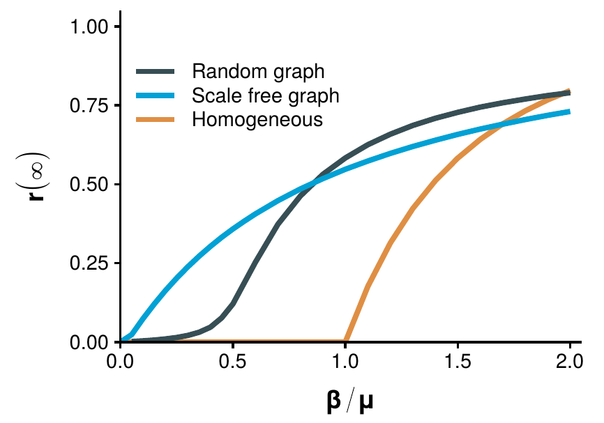
Figure 3.9: Epidemic threshold and topology. Total fraction of recovered individuals in equilibrium conditions as a function of \(\beta/\mu\). In the homogeneous mixing approach the epidemic threshold is 1. When the SIR model is implemented in a random network with \(\langle k \rangle = 3\) the epidemic threshold is \(1/3\) (3.71). Conversely, in a SF network with \(\langle k \rangle = 3\) and \(\langle k^2 \rangle = 113\) the epidemic threshold is \(0.03\). Note that the size of the network is \(N=10^4\), with a maximum degree of \(k_\text{max} = \sqrt{N}\) to avoid correlations (see chapter 2). Hence, the threshold does not vanish completely, as it is supposed to be 0 only the limit of \(N\rightarrow \infty\).

Furthermore, note that to obtain expression (3.67) the only property of the network that we have used is that it is uncorrelated. Whence, it can be used to study any network that we desire. In particular, in the case of random graphs the degree distribution is Poisson, implying that \(\langle k^2 \rangle = \langle k \rangle^2 + \langle k \rangle\). Thus, for those networks the epidemic threshold is simplified to

\[\begin{equation} R_0 = \frac{\beta}{\mu} > \frac{1}{\langle k \rangle + 1}\,, \tag{3.69} \end{equation}\]

which is the result obtained by the earliest studies of gonorrhea propagation (3.53) (except for the \(+1\), but its role will be elucidated in a moment). In other words, we can say that the problem in those models is that they implicitly assumed a random contact network when they should have used a scale free network instead. In figure 3.9 we show a comparison of the final size of the epidemic as a function of \(R_0\) between ER networks, SF networks and the homogeneous mixing approach.

Note that most of the ideas had been around for years, but did not get that much attention. We could argue that what really made the difference in the case of the work by Pastor-Satorras and Vespignani was the use of data. Indeed, many theoretical approaches can be proposed, but without experimental data it is not possible to really gauge their importance. Thus, once again, this highlights how incorporating more data into already existing models can make the difference.

To conclude, we should address why the equation obtained by Anderson and May for the SIR model did not have a \(-1\) factor (3.57), the one from Andersson also for the SIR model did (3.59) and the one from Pastor-Satorras and Vespignani for the SIS model did not (3.67). The first observation is that in the SIS model on a network, it is possible that if \(i\) infects \(j\), then \(i\) recovers and \(j\) infects \(i\). This cannot happen in the SIR model, so for a node of degree \(k\) only \(k-1\) links can transmit the disease,

\[\begin{equation} \Theta = \sum_k \frac{(k-1)P(k)\rho_k}{\sum_s s P(s)}\,, \tag{3.70} \end{equation}\]

leading to the threshold [243]

\[\begin{equation} R_0^\text{SIR} > \frac{\langle k \rangle}{\langle k^2\rangle - \langle k \rangle}\,. \tag{3.71} \end{equation}\]

Which explains the discrepancy between (3.59) and (3.67). Lastly, note that in the case of Anderson and May they did not consider a fixed structure, such as a network, but rather that at each time step every individual would seek \(i\) new sexual partners. Thus, the correction accounting where the disease came from does not apply to their model.

3.3.2 The generating function approach

There are multiple techniques that can be used to solve the system (3.61) and obtain the value of the epidemic threshold (see [145], [243] for a review). In this section we will describe an approach introduced by Newman in 2002 inspired by percolation [244], based on the use of generating functions, that is specially suited to analyze directed networks. This is the methodology that we will use in section 3.3.3 to study disease propagation in directed multiplex networks.

Although for the moment we are only interested in undirected networks, we will introduce the methodology considering that the networks might have both directed and undirected links [245], as this will be the approach used in section 3.3.3. Hence, suppose that the probability that a random node of the network has \(j\) incoming links, \(l\) outgoing links and \(m\) undirected links is \(p_{jlm}\). The generating function of the distribution will be

\[\begin{equation} G(x,y,z) = \sum_{j=0}^\infty \sum_{l=0}^\infty \sum_{m=0}^\infty p_{jlm} x^j y^l z^m\,. \tag{3.72} \end{equation}\]

As long as \(p_{jlm}\) is normalized this function has the property \(G(1,1,1) = 1\) and

\[\begin{equation} \langle k_d \rangle = \frac{\text{d}G(1,1,1)}{\text{d}x} \equiv G^{(1,0,0)}(1,1,1)\,, \tag{3.73} \end{equation}\]

where \(\langle k_d \rangle\) is the average number of incoming links in the network. As for any incoming link there has to be also an outgoing link,

\[\begin{equation} \langle k_d \rangle = \frac{\text{d}G(1,1,1)}{\text{d}y} \equiv G^{(0,1,0)}(1,1,1) = G^{(1,0,0)}(1,1,1)\,. \tag{3.74} \end{equation}\]

Lastly, for the undirected links

\[\begin{equation} \langle k_u \rangle = \frac{\text{d}G(1,1,1)}{\text{d}z} \equiv G^{(0,0,1)}(1,1,1)\,. \tag{3.75} \end{equation}\]

A related quantity that will be needed for the derivation is the generating function of the excess degree distribution, which is the degree distribution of nodes reached by following a randomly chosen link, without considering the one we came along. Note that if we choose a node at random, its degree will depend on \(p_k\), however if we follow a link the probability will be higher the more links the node has, \(k p_k\). Thus, the generating function obtained by following a directed link is

\[\begin{equation} H_d(x,y,z) = \frac{\sum_{jlm} j x^{j-1} y^l z^m}{\sum_{jkm} j p_{jlm}} = \frac{1}{\langle k_d \rangle} G^{(1,0,0)}(x,y,z)\,, \tag{3.76} \end{equation}\]

similarly if we follow a directed link in the reverse direction,

\[\begin{equation} H_r(x,y,z) = \frac{\sum_{jlm} l x^{j} y^{l-1} z^m}{\sum_{jkm} l p_{jlm}} = \frac{1}{\langle k_d \rangle} G^{(0,1,0)}(x,y,z)\,, \tag{3.77} \end{equation}\]

and lastly if we follow an undirected link,

\[\begin{equation} H_u(x,y,z) = \frac{\sum_{jlm} m x^{j} y^l z^{m-1}}{\sum_{jkm} m p_{jlm}} = \frac{1}{\langle k_u \rangle} G^{(0,0,1)}(x,y,z)\,. \tag{3.78} \end{equation}\]

The next step is to take into account that the disease will not be transmitted through all the links. Indeed, we define the probability of a link “being infected” in the sense that node \(i\) transmits the disease to \(j\) using that link as \(T\) (regardless of it being directed or undirected). Hence, the probability of a node having exactly \(a\) of the \(j\) links emerging from it infected is given by the binomial distribution \(\binom{j}{a} T^a(1-T)^{j-a}\). Under these assumptions, the generating function is modified so that

\[\begin{equation} \begin{split} G(x,y,z;T) & = \sum_{jlm} p_{jlm} \left[ \sum_{a=0}^j \dbinom{j}{a} (Tx)^a (1-T)^{j-a} \sum_{b=0}^l \dbinom{l}{b} (Ty)^b (1-T)^{l-b}\right. \\ & \left. ~~~~~~~~~~~~~~~\sum_{c=0}^m \dbinom{m}{c} (Tz)^c(1-T)^{m-c}\right] \\ & = \sum_{jlm} p_{jlm} (1-T+Tx)^j (1-T+Ty)^l (1-T+Tz)^m \\ & = G(1+(x-1)T,1+(y-1)T,1+(z-1)T)\,. \end{split} \tag{3.79} \end{equation}\]

Analogously, the generating functions for the distribution of infected links of a node reached by following randomly chosen links are:

\[\begin{equation} \begin{split} H_f(x,y,z;T) & = H_f(1+(x-1)T,1+(y-1)T,1+(z-1)T) \\ H_r(x,y,z;T) & = H_r(1+(x-1)T,1+(y-1)T,1+(z-1)T) \\ H_u(x,y,z;T) & = H_u(1+(x-1)T,1+(y-1)T,1+(z-1)T)\,. \end{split} \tag{3.80} \end{equation}\]

The fundamental quantity that we want to obtain is the number \(s\) of nodes contained in an outbreak that begins at a randomly selected node. Let \(g(w,T)\) be the generating function for the probability that a randomly chosen node belongs to a group of infected nodes of a given size:

\[\begin{equation} g(w;T) = \sum_s P_s(T) w^s\,. \tag{3.81} \end{equation}\]

To solve it, we also need to evaluate the probability that a randomly chosen link leads to a node belonging to a group of infected nodes of given size. The generating function of the distribution reads

\[\begin{equation} h_d(w;T) = \sum_t P_t(T) w^t\,. \tag{3.82} \end{equation}\]

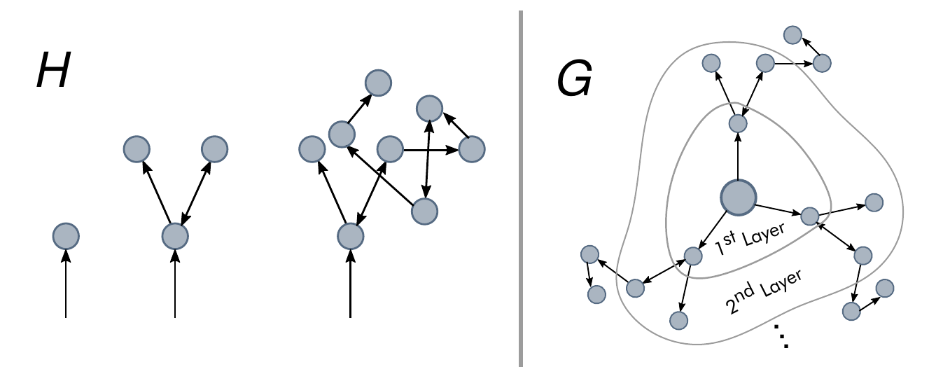
Figure 3.10: Scheme of the generating function approach. Left: The generating function of the excess degree, \(H\), gives the distribution of links (directed and undirected) of a node reached by following a random link. Right: As the infection starts in a node, the generating function of the node’s degree, \(G\), has to be used. Hence, \(G(H(x))\) gives the distribution of links in the first layer, \(G(H(H(x))\) in the second layer, etc.

This expression satisfies a condition of the form

\[\begin{equation} h_d(w;T) = w H_d(1,h_d(w;T),h_u(w;T))\,. \tag{3.83} \end{equation}\]

Similarly, in the case of undirected links,

\[\begin{equation} h_u(w;T) = w H_u(1,h_d(w;T),h_u(w;T))\,. \tag{3.84} \end{equation}\]

With the expressions (3.80) and these two last equations, we have completely defined the distribution of \(t\). It follows (see figure 3.10) that if the disease starts at a randomly chosen node the distribution is

\[\begin{equation} g(w;T) = w G(1,h_d(w;T),h_u(w;T))\,, \tag{3.85} \end{equation}\]

yielding an average size of outbreaks of

\[\begin{equation} \langle s \rangle = \sum_s s P_s(T) = \left.\frac{\text{d}g(w;T)}{\text{d}w} \right|_{w=1}\,. \tag{3.86} \end{equation}\]

Performing the derivatives and setting \(w=1\) we obtain

\[\begin{equation} \begin{split} g' & = 1 + G^{(0,1,0)} h_d' + G^{(0,0,1)} h_u'\\ h_d' & = 1 + H_d^{(0,1,0)} h_d' + H_d^{(0,0,1)} h_u' \\ h_u' & = 1 + H_u^{(0,1,0)} h_d' + H_u^{(0,0,1)} h_u'\,, \end{split} \tag{3.87} \end{equation}\]

where we have dropped the arguments of the functions for readability. Inserting these equations in (3.86) we obtain

\[\begin{equation} \begin{split} \langle s \rangle = 1 & + \frac{G^{(0,1,0)} \left(1-H^{(0,1,0)}_d + H_u^{(0,1,0)}\right)}{\left(1-H_d^{(0,1,0)}\right)\left(1-H_u^{(0,0,1)}\right) - H_u^{(0,1,0)}H_d^{(0,0,1)}} \\ & + \frac{G^{(0,0,1)} \left(1-H^{(0,0,1)}_d + H_u^{(0,0,1)}\right)}{\left(1-H_d^{(0,1,0)}\right)\left(1-H_u^{(0,0,1)}\right) - H_u^{(0,1,0)}H_d^{(0,0,1)}} \,. \end{split} \tag{3.88} \end{equation}\]

Note that this expression diverges if

\[\begin{equation} \left(1-H_d^{(0,1,0)}\right)\left(1-H_u^{(0,0,1)}\right) - H_u^{(0,1,0)}H_d^{(0,0,1)} = 0\,. \tag{3.89} \end{equation}\]

In other words, equation (3.89) sets the condition for the epidemic threshold. The last step is to note that

\[\begin{equation} G^{(1,0,0)} (1,1,1;T) = T G^{(1,0,0)}(1,1,1)\,, \tag{3.90} \end{equation}\]

and similarly for the rest of equations. Hence, equation (3.89) reads

\[\begin{equation} \left(1-T H_d^{(0,1,0)}\right)\left(1-T H_u^{(0,0,1)}\right) - T^2 H_u^{(0,1,0)}H_d^{(0,0,1)} = 0\,, \tag{3.91} \end{equation}\]

where now the arguments of the functions are \((1,1,1)\) instead of \((1,1,1;T)\).

In the particular case of undirected networks this expression further simplifies to

\[\begin{equation} 1 - T H_u^{(0,0,1)} = 0 \Rightarrow T = \frac{1}{H_u^{(0,0,1)}}\,. \tag{3.92} \end{equation}\]

To rewrite this expression in a more familiar format we can calculate the explicit dependency of \(H_u^{(0,0,1)}\) as a function of the network topology:

\[\begin{equation} \begin{split} H_u^{(0,0,1)}(1,1,1) & = \frac{1}{\langle k \rangle}\frac{\text{d}}{\text{d}z} G^{(0,0,1)} (1,1,1) = \frac{1}{\langle k \rangle} \frac{\text{d}^2}{\text{d}z^2} \left.\sum_m p_m z^m \right|_{z=1}\\ & = \frac{1}{\langle k \rangle} \sum_m m(m-1) p_m = \frac{1}{\langle k \rangle} \left(\langle k^2 \rangle - \langle k \rangle \right) \,. \end{split} \tag{3.93} \end{equation}\]

Therefore, the epidemic threshold is

\[\begin{equation} T = \frac{\langle k \rangle}{\langle k^2 \rangle - \langle k \rangle}\,. \tag{3.94} \end{equation}\]

3.3.3 Directionality reduces the epidemic threshold in directed multiplex networks

And the “cosmological principles” were, I fear, dogmas that should not have been proposed.
Karl Popper

As we saw in chapter 2, network science constitutes a whole field of research on its own. Therefore, any advance in the understanding of networks in general might also have its applications in the study of disease spreading on networks. In particular, we can investigate the dynamics of diseases on the multilayer networks we introduced in section 2.1.3 [246]. One option can be to have the same network pattern in all layers but different dynamics on each of them, such as modeling the spreading of two interacting diseases in the same population [247] or the interplay between information and disease spreading that we discussed in the introduction [248]. On the other hand, we can have the same dynamics in all layers but diverse interaction patterns in each of them, in a similar fashion as our model of section 3.2.3.

In this work we will focus on the latter, i.e., the same dynamics in the whole system but different networks in the layers. Even more, we will consider that the networks can have directed links, something that is usually disregarded in epidemic models (note that adding direction to links implies that more data is necessary than just knowing that there is a relationship between two agents). Some relevant examples of the importance of the directionality in this context are the case of meerkats in which transmission varies between groomers and groomees [249] and even in the transmission of HIV that we have briefly discussed, as male-to-female transmission is 2.3 times greater than female-to-male transmission [117]. Similarly, when addressing the problem of diseases that can be transmitted among different species, it is important to account for the fact that they might be able to spread from one type of host to the other, but not the other way around. For instance, the bubonic plague can be endemic in rodent populations and spread to humans under certain conditions. If it evolves to the pneumonic form, it may then spread from human to human [250]. Analogously, Andes virus spreads within rodent populations, but it can be transmitted to humans and then spread via person-to-person contacts [251].

Recall that in multilayer networks there are two types of links: intralayer (those contained within layers) and interlayer (those connecting nodes set in different layers). Our objective is to understand how the epidemic threshold is influenced by the directionality of both intralayer and interlayer links. In particular, we will consider multiplex networks composed by two layers with either homogeneous or heterogeneous degree distributions in the layers (i.e., ER or SF networks). Besides, we will analyze several combinations of directionality: (i) Directed layer - Undirected interlinks - Directed layer (DUD); (ii) Directed layer - Directed interlinks - Directed layer (DDD); and Undirected layer - Directed interlinks - Undirected layer (UDU). For the sake of comparison, we will also include the standard scenario, namely, (iv) Undirected layer - Undirected interlinks - Undirected layer (UUU). We will implement a susceptible-infected-susceptible (SIS) model on these networks and study the evolution of the epidemic threshold as a function of the directionality and the coupling strength between layers. In addition, we will derive analytically the epidemic threshold using generating functions (see 3.3.2) to obtain theoretical insights on the underlying mechanisms driving the dynamics of these systems.

First, we implement stochastic SIS dynamics on the two layer multiplex networks. Note that as there are two types of links, we can associate a different spreading probability to each of them: the interlayer spreading probability, \(\gamma\), and the intralayer spreading probability, \(\beta\) [252]. Accordingly, a node can transmit the disease with probability \(\beta\) to those susceptible neighbors contained in the same layer and with probability \(\gamma\) to those set in the other layer. As a consequence, the epidemic threshold will depend on both parameters. Thus, henceforth we will define the epidemic threshold as \(\beta_c\) and explore its value as a function of \(\gamma\) (note that previously we defined the epidemic threshold as the ratio \(\beta/\mu\), but in this case we will keep fixed the value of \(\mu\) for simplicity).

In the simulations, all the nodes are initially susceptible. The spreading starts when one node is set to the infectious state. Then, at each time step, each infected node spreads the disease through each of its links with probability \(\beta\) if the link is contained in a layer and with probability \(\gamma\) if the link connects nodes in different layers. Besides, each infected node recovers with probability \(\mu\) at each time step. The simulation runs until a stationary state for the number of infected individuals is reached.

To determine the epidemic threshold we fix the value of \(\gamma\) and run the simulation over multiple values of \(\beta\), repeating \(10^3\) times the simulation for each of those values. The minimum value of \(\beta\) at which, on average, the number of infected individuals in the steady state is greater than one determines the value of the epidemic threshold. This procedure is then repeated for several values of \(\gamma\) to obtain the dependency of \(\beta_c\) with the spreading across layers. Lastly, this dependency is evaluated for \(100\) realizations of each network considered in the study and their \(\beta_c(\gamma)\) curves are averaged.

For the cases in which the interlinks are directed, we need to add another parameter to the model. If all the links were to point in the same direction, the epidemic threshold would be trivially the one of the source layer and thus the multiplex structure would play no role. For this reason, for each directed link connecting layers \(u\) and \(v\) we set the directionality to be \(u\rightarrow v\) with probability \(p\) and \(u\leftarrow v\) with probability \((1-p)\). Consequently, in networks with directed interlinks the epidemic threshold will be given as a function of this probability \(p\).

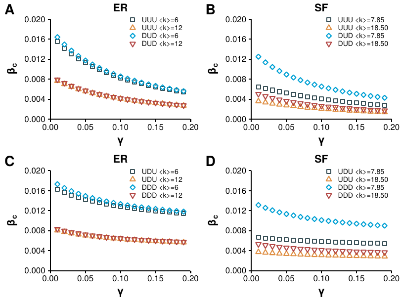
Figure 3.11: Epidemic threshold in directed multilayer networks according to SIS simulations. Several configurations of networks are considered: A) ER networks with undirected interlinks; B) SF networks with undirected interlinks; C) ER networks with directed interlinks; D) SF networks with directed interlinks. In all cases \(\mu=0.1\) the number of nodes is \(N=2\cdot 10^4\) and for each directionality configuration there are two sets of networks with different average degree as shown in the legend. In the networks with directed interlinks \(p=0.5\).

The results, figure 3.11, signal that the consequences of changing the directionality of some links is completely different for SF and ER networks. In particular, in 3.11A, we can see that for networks with \(\langle k \rangle = 6\) the epidemic threshold is very similar in both UUU and DUD configurations. This effect is again seen for denser networks, \(\langle k \rangle = 12\), implying that it is the directionality of the interlinks, and not the one of the links contained within layers, the main driver of the epidemic in these networks. On the other hand, in figure 3.11B we can see that this behavior is not replicated in SF networks. Certainly, there is a large difference between the curves of the UUU and DUD configurations, implying that the directionality of intralinks is much more important in this type of networks. A similar pattern is observed in figures 3.11C and 3.11D, in which the interlinks are directed. Moreover, in all the cases considered the epidemic threshold is always lower for those configurations with undirected links within the layers, compared to those in which those links are directed, given the same interlink directionality.

To get further insights into the mechanisms driving this behavior we proceed to compute analytically the epidemic threshold. We introduced the generating function of the network, equation (3.72), saying that it accounts for the probability of having \(j\) incoming links, \(l\) outgoing links and \(m\) undirected links. However, in this case the directionality of links within the layers is always the same (we do not mix directed and undirected links). Hence, we can use \(j\) as an indicator for directed links when we have directed intralinks, or we can regard it as the number of undirected links otherwise. This frees \(m\) to be used for the interlinks. In other words, the generating function will now be \(G(x,z)\) if the network has the shape UXU and \(G(x,y,z)\) if it is DXD, with \(z\) representing the links connecting different layers.

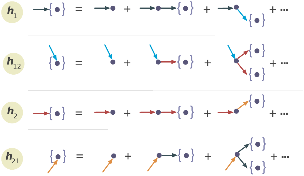
Figure 3.12: Scheme of the generating function on multilayer networks. Recursive relation of generating functions for the size distribution of outbreaks by following a link in layer 1, \(h_1\), from 1 to 2, \(h_{12}\), in layer 2, \(h_2\), and from 2 to 1, \(h_{21}\).

Analogously, the definition of the generating function for the excess distribution (3.76) does not change. The first difference is encountered when we want to obtain the probability of a link being infected. In the previous case, we set said probability equal to \(T\) in all links, but now we have \(\beta\) for links within layers and \(\gamma\) for links across layers. Thus, we keep \(T\) as the probability of a link within layers being infected, and denote the probability of the other set of links being infected as \(T_{uv}\). With these definitions equation (3.79) now reads

\[\begin{equation} G(x,y,z;T,T_{uv}) = G(1+(x-1)T,1+(y-1)T,1+(z-1)T_{uv})\,. \tag{3.95} \end{equation}\]

Next, we introduced the generating function used to calculate the probability that a randomly chosen link belongs to the group of infected nodes. We distinguished \(h_d\) and \(h_u\) if the links were directed or undirected respectively. In this case, as the directionality is the same, what we need to define is \(h_1\) if the link is in layer \(1\), \(h_2\) if it is in layer 2, \(h_{12}\) if it is a link going from layer 1 to layer 2 and \(h_{21}\) if it is going from layer 2 to layer 1. The recursive relations in this case (see figure 3.12) read

\[\begin{equation} \begin{split} h_1(w;T,T_{uv}) & = wH_1(1,h_1(w;T,T_{uv}),h_{12}(w;T,T_{uv});T,T_{uv}) \\ h_2(w;T,T_{uv}) & = wH_2(1,h_2(w;T,T_{uv}),h_{21}(w;T,T_{uv});T,T_{uv}) \\ h_{12}(w;T,T_{uv}) & = wH_{12}(1,h_2(w;T,T_{uv}),h_{21}(w;T,T_{uv});T,T_{uv}) \\ h_{21}(w;T,T_{uv}) & = wH_{21}(1,h_1(w;T,T_{uv}),h_{12}(w;T,T_{uv});T,T_{uv}) \,. \end{split} \tag{3.96} \end{equation}\]

Then, the generating function for the distribution of the size of an outbreak starting in a randomly chosen node in layer 1 is

\[\begin{equation} g(w;T,T_{uv}) = wG(1,h_1(w;T,T_{uv}),h_{12}(w;T,T_{uv});T,T_{uv})\,. \tag{3.97} \end{equation}\]

Leading to the expression of the average size of an outbreak:

\[\begin{equation} \begin{split} \langle s \rangle & = \sum_s s P_s(T) = \left.\frac{\text{d}g(w;T,T_{uv})}{\text{d}w}\right|_{w=1} \\ & = 1 + G^{(0,1,0)}h_1' + G^{(0,0,1)}h_{12}'\,. \end{split} \tag{3.98} \end{equation}\]

As in the previous case, this equation diverges when the denominator is equal to 0. Hence, after some algebra, the condition that establishes the epidemic threshold reads

\[\begin{equation} \begin{split} 0 = & \left[\left(1-H_1^{(0,1,0)}\right) \left(1-H_{12}^{(0,0,1)}H_{21}^{(0,0,1)}\right)-H_1^{(0,0,1)}H_{12}^{(0,0,1)}H_{21}^{(0,1,0)}\right] \\ & \cdot \left[\left(1-H_2^{(0,1,0)}\right)\left(1-H_{12}^{(0,0,1)}H_{21}^{(0,0,1)}\right) - H_2^{(0,0,1)}H_{21}^{(0,0,1)}H_{12}^{(0,1,0)}\right] \\ & - H_1^{(0,0,1)}H_2^{(0,0,1)} H_{12}^{(0,1,0)} H_{21}^{(0,1,0)}\,. \end{split} \tag{3.99} \end{equation}\]

Note that this expression works for all the configurations we are considering in this work, given that we choose the proper values of \(H_x\). For instance, for the DUD configuration we have

\[\begin{equation} \begin{split} & H_1^{(0,1,0)} = H_2^{(0,1,0)} = T\langle k \rangle \\ & H_1^{(0,0,1)} = H_2^{(0,0,1)} = T \langle k \rangle \\ & H_{12}^{(0,1,0)} = H_{21}^{(0,1,0)} = T_{uv} \\ & H_{12}^{(0,0,1)} = H_{21}^{(0,0,1)} = T_{uv}\, \end{split} \tag{3.100} \end{equation}\]

yielding

\[\begin{equation} \tag{ER-DUD} T_c = \frac{1-T_{uv}}{\langle k \rangle}\,. \end{equation}\]

Similarly, we can obtain the epidemic threshold for the rest of the configurations:

\[\begin{equation} \tag{ER-UUU} T_c = \frac{1-T_{uv}}{\langle k \rangle + 1 - T_{uv}}\,, \end{equation}\]

\[\begin{equation} \tag{ER-DDD} T_c = \frac{2}{\langle k \rangle ( 2 + m + \sqrt{m(m+8)})}\,, \end{equation}\]

where \(m = p(1-p) T_{uv}^2\),

\[\begin{equation} \tag{ER-UDU} T_c = \frac{2(1+\langle k \rangle ) + m' - \sqrt{m'(4+8\langle k \rangle +m')}}{2((1+\langle k \rangle)^2 -m' \langle k \rangle)}\,, \end{equation}\]

with \(m'=\langle k \rangle p (1-p) T_{uv}^2\). These results were simplified thanks to the property \(\langle k^2\rangle = \langle k \rangle^2 + \langle k \rangle\) of Poisson distributions. For the case of SF, on the other hand, we cannot do this simplification and thus some expressions will depend on both moments of the distribution:

\[\begin{equation} \tag{DUD-SF} T_c = \frac{1-T_{uv}}{\langle k \rangle}\,, \end{equation}\]

\[\begin{equation} \tag{UUU-SF} T_c = \frac{\langle k \rangle (1-T_{uv})}{\langle k^2\rangle (1-T_{uv}) + \langle k \rangle^2 T_{uv}}\,, \end{equation}\]

\[\begin{equation} \tag{DDD-SF} T_c = \frac{2}{\langle k \rangle (2+m+\sqrt{m(m+8)})}\,, \end{equation}\]

where \(m = p(1-p) T_{uv}^2\), and lastly

\[\begin{equation} \tag{UDU-SF} T_c = \frac{2\langle k^2\rangle \langle k \rangle + \langle k \rangle^2\left(\langle k \rangle m - \sqrt{m(4\langle k^2\rangle + \langle k \rangle^2(4+m))}\right)}{2(\langle k ^2\rangle^2 - \langle k \rangle^4m)}\,. \end{equation}\]

These expressions closely match the results obtained in the simulations, figure 3.13. Again, we can observe that the value of the epidemic threshold of the DUD configuration in SF networks tends to the value of the UUU configuration for large values of the spreading probability across layers, mimicking the behavior of ER networks. Hence, in general, we can conclude that the directionality (or lack of) of the interlinks is the main driver of the epidemic spreading process. The exception is the limit of small spreading from layer to layer as in this scenario the directionality of interlinks makes SF networks much more resilient. Altogether, the conclusion is that directionality reduces the impact of disease spreading in multilayer systems.

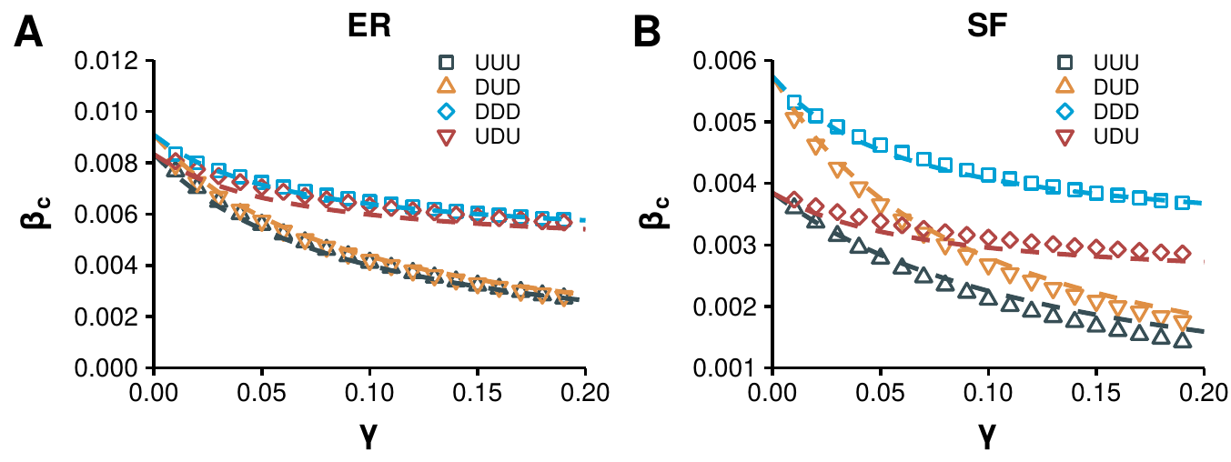
Figure 3.13: Epidemic threshold in directed multilayer networks, simulations vs. theory. A) Comparison between the results of the stochastic simulations (points) and the theoretical predictions (lines) for the ER set of networks. B) As A) but for SF networks.

It is worth point out that these results are not only relevant for the situations we have described in this chapter so far. One particularly interesting and open challenge is to quantify the effects that the interplay between different social networks could have on spreading dynamics. The theoretical framework developed here is particularly suited to study this and similar challenges related to the spreading of information in social networks. On one hand, because social links are not always reciprocal [253], specially in online systems in which a user is not necessarily followed by her followings. Besides, disease-like models have been widely used to study information dissemination [246], [254]. For this reason, we have analyzed the dependence of the epidemic threshold with the inter-spreading rate in a real social network composed by two layers, figure 3.14A. The first layer of the multilayer system is made up by the directed set of interactions in a subset of users of the now defunct FriendFeed platform, whereas the second layer is defined by the directed set of interactions of those same users in Twitter. Even though this multiplex network corresponds to a DUD configuration, we have also explored the other configurations that we have studied. Note that in contrast to the synthetic networks used so far, in this network the layers have different average degree. In particular, the FriendFeed layer has 4,768 nodes and 29,501 directed links, resulting in an average out-degree of 6.19 while the Twitter layer is composed by 4,786 nodes and 40,168 directed links, with an average out-degree of 8.42. Nevertheless, their degree distributions are both heavy tailed, resembling the power law structure of SF networks, although the maximum degree in the FriendFeed network is much larger than in the Twitter network [255].

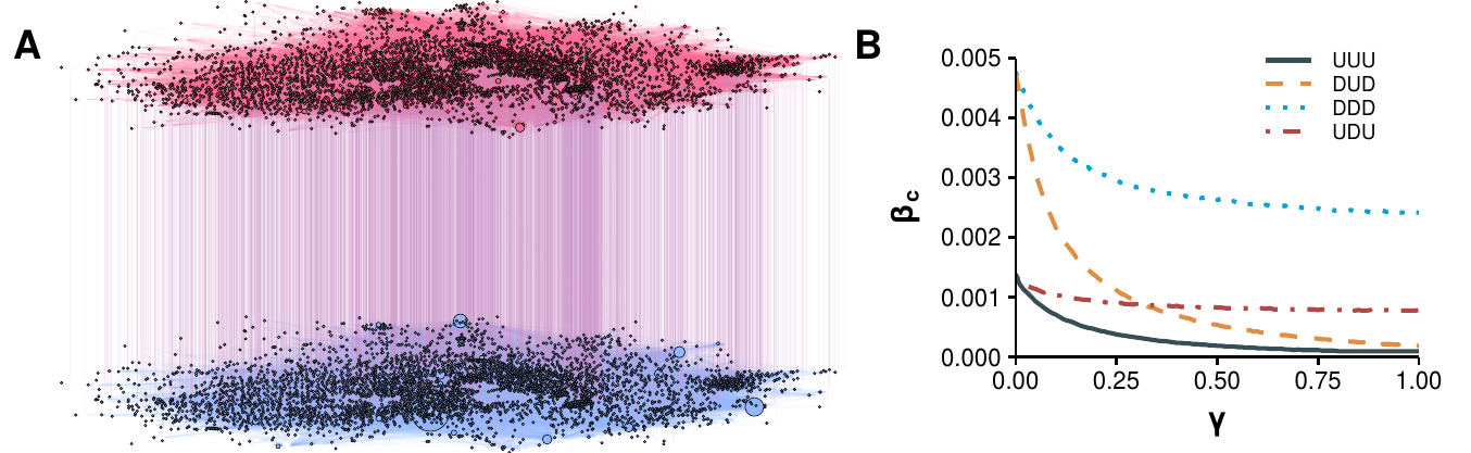
Figure 3.14: Epidemic threshold in a multilayer social system. Epidemic threshold obtained from simulations in a multiplex network composed by users of two different social platforms: FriendFeed and Twitter. The original network, panel A, has directed intralinks and undirected interlinks, corresponding to a DUD configuration. Nevertheless, to explore the effects of directionality in a real scenario, the four discussed configurations are considered in panel B. For those configurations with directed interlinks we set \(p=0.5\).

The results, figure 3.14B, confirm the findings of synthetic networks. In particular, configurations with some directionality are always more resilient against the spreading. Consequently, information travels much more easily in undirected systems than in directed systems. This is particularly worrisome given that even though Twitter can be modeled as a directed network, social networks such as Facebook and Whatsapp should be modeled using undirected configurations and, recently, these two platforms were identified as one of the main sources of misinformation spreading [256].

In summary, we have seen the importance that networks have in shaping disease dynamics. Hence, as more data becomes available, our network models should be improved in order to better account for the real mechanisms behind such a dynamics. To this end, in this section we have developed a framework that allows studying disease-like processes in multilayer networks with, possibly, directed links. This represents an important step towards the characterization of diffusion processes in interdependent systems. Our results show that directionality has a positive impact on the system’s resistance to disease propagation. Furthermore, we have seen that the way in which interconnected social networks are coupled can determine their ability to spread information. Hence, the insights obtained in this work can be applied to a plethora of systems and show that more emphasis should be put in studying the role of interlinks and directionality in diffusion processes.

3.4 Age and network structures

The problems that we have studied in this chapter have shown us that, when we consider no longer that humans are particles, the dynamics of an epidemic can change dramatically. Note that the mass action approximation was just a handy tool to overcome either the scarcity of data in the past or the analytical intractability of some formulations. However, nowadays we have both enough data and computational power to introduce many more details in the dynamics.

It is now time to return to where we left at the end of chapter 2. In section 2.6.3 we introduced a mathematical framework that allowed us to create networks in which both the degree distribution and the age contact patterns of the population could be taken into account. With all the information we have gathered about disease dynamics, we can finally analyze the implications of this choice.

In the following, we will consider four different scenarios depending on the data that one may have at her disposal:

1. Homogeneous mixing with \(\langle C \rangle\): suppose that the only data available is the average number of contacts and individual may have. In this case, we would be in the same situation as in the studies of gonorrhea that we presented in section 3.3. According to equation (3.53) the epidemic threshold in this situation is

\[\begin{equation} \frac{\beta}{\mu} = \frac{1}{\langle C \rangle}\,. \end{equation}\]

2. Homogeneous mixing with age contact patterns: if data about the mixing patterns of the population is available, we can improve the model by creating multiple homogeneous mixing groups, one for each age bracket, as we discussed in section 3.1.1. Note that this formulation is similar to the one that Anderson and May introduced for studying interacting groups with different activity patterns, equation (3.54). Hence, the epidemic threshold, according to equation (3.57), should be

\[\begin{equation} \frac{\beta}{\mu} = \frac{\langle C \rangle}{\langle C^2 \rangle}\,. \end{equation}\]

3. Network information: if we have only information about the network structure, the epidemic threshold is given by (3.71),

\[\begin{equation} \frac{\beta}{\mu} = \frac{\langle k \rangle}{\langle k^2\rangle - \langle k \rangle}\,. \end{equation}\]

4. Network and age information: if we are able to obtain information about both the network structure and the age mixing patterns of the population, we can build the network of interactions using the techniques introduced in section 2.6.3.

Figure 3.15: Phase diagram for different amounts of data. We compare the total number of recovered individuals as a function of the ratio \(\beta/\mu\) for four models, each one determined by the amount of data used. In the homogeneous scenario the only information is \(\langle C\rangle = 6.18\) which yields an epidemic threshold of approximately \(0.16\). Next, we extract the information about the age mixing patterns of Belgium in 2005 from the polymod study [131] and weight the matrix so that the average number of contacts is also \(6.18\). This, in turn, produces \(\langle C^2\rangle = 40.37\) yielding an epidemic threshold slightly over \(0.15\). To model the network structure we have assumed that the degree distribution follows a power law with \(\langle k \rangle = 6.18\) and \(\langle k^2\rangle = 102.27\), resulting in a threshold of \(0.06\). Lastly, we have combined this network distribution with the data from Belgium to build the age contact network.

To properly compare the four situations we will set in all of them the same average number of contacts, which we denote by \(\langle C\rangle\) when there is no network information and by \(\langle k \rangle\) when there is. Next, we perform numerical simulations of these scenarios, using the SIR model introduced so far (with the adequate modifications depending on the amount of data available), to compare the evolution of the epidemic size as a function of the ratio \(\beta/\mu\), figure (fig:chap3-age-comparison).

We can clearly see the effect that the heterogeneity of the network introduces in the system. For the homogeneous scenario and the homogeneous with information about the mixing patterns, the epidemic threshold is almost the same. However, when we introduce a network with a power law degree distribution, the heterogeneity in the contacts is much larger, yielding a smaller epidemic threshold. Thus, it seems that from this point of view it is more important to be able to collect data about the contact structure of the population than from the age mixing patterns.

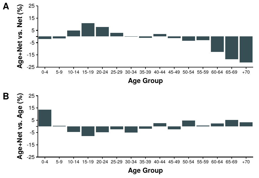
Figure 3.16: Comparison of attack rate per age group. In A we compare the number of recovered individuals in each age bracket in the model with age and network structure against the model with information of the network structure, so that positive values imply that the attack was larger in the model with more information, and vice versa. In B the comparison is done between the model with all the information and the homogeneous with age mixing patterns. Note that to compare similar situations a value of \(\beta=0.21\) has been chosen, as it is the value in which the three dynamics intersect in figure 3.15.

On the other hand, note that there are many diseases which can affect differently an individual depending on her age. This effect was particularly important, for instance, in the 2009 H1N1 pandemic [257]. Furthermore, age is one of the factors used to classify people into risk groups, which in turn are the main targets of vaccination campaigns. Hence, even if, according to figure 3.15, knowledge of the age structure does not seem too important, once we look closer into the dynamics of the system the situation changes.

To illustrate this, in figure 3.16, we compare the attack rate of each group in the different models. In particular, in panel A we show the relative change on the amount of recovered individuals per age group between the model with all the information and the model that only considers the network structure. As we can see, the complete model has higher attack rates in teenagers, while having much lower attack rates among the elderly. Thus, even if the total attack rate in both situations is the same, if the decision to administer a vaccine is only based on the network structure we would be making a big mistake.

Conversely, adding the network information to the age mixing matrices has a smaller effect, indicating that from this point of view it is more important to collect data about the age mixing patterns of the population than from the network structure. Note that the network structure in these models is not extracted from data. Hence, the differences that we can see in panel B do not have any specific interpretation rather than that the power law distribution that we chose is responsible for those differences.

To summarize, it is clear that the more data we have, the better, as long as we use it properly and fully understand it. Yet, if for some reason we need to choose which data we need to collect, it is important to know the final application, as it is not straightforward to say which information is more valuable. In particular, we have seen that the network structure has dramatic effects on both the epidemic threshold and the incidence of the epidemic. But, on the other hand, having information about the mixing patterns of the population might be more valuable in some situations, such as determining risk groups for vaccination.

---

8. A noteworthy exception is the work by Daniel Bernoulli in 1766, although he was just too ahead of his time. Furthermore, some authors claim that the credit for creating the first modern disease transmission model should go to Pyotr Dimitrievich Enko. Unfortunately, even though he published his work as early as 1889, he wrote it in russian and thus it became largely unnoticed for the majority of the scientific community until it was translated by the middle of the XX century (see [140], [141] for a nice introduction to the early days of mathematical epidemiology).↩︎

9. A metapopulation is a set of populations that are spatially separated but can exchange individuals. Within each subpopulation any plausible disease dynamics can be implemented, although usually the homogeneous mixing approach is used [172].↩︎

10. In the original paper at a certain point the authors expand a quantity using Taylor’s theorem an introduce the notation \(R_n = \int_0^\infty a^n p(a) m(a) \text{d}A\). Then, they determine the ratio between the total births in two successive generations to be \(\int_0^\infty p(a) m(a) \text{d} A\), which is equal to \(R_0\) according to the previous definition. Thus, the subscript \(0\) historically would represent the \(0\)-\(th\) moment of the distribution. In modern literature, however, the subscript is interpreted as referring to the “very beginning” of the epidemic [140]. Note also that \(R_0\) is usually pronounced R naught in Britain and R zero in the U.S. [187].↩︎

11. Although the notation \(R_0\) is well established, there is not an agreement on how to call this quantity. Exchanging the word reproduction for reproductive is common in the literature, as well as using rate or ratio instead of number. Although the differences are minimal, note that rate is clearly wrong as it is not a rate but a (dimensionless) ratio [191].↩︎

12. Even though we have not discussed yet on how to introduce networks in epidemic modeling, note that an homogeneous population is equivalent to a complete network in which every node is connected to every other node. Hence, these overlapping structures can also be regarded as a multiplex network in which each node can be in more than one layer↩︎

13. Actually, the shape of the distribution was the same as the ones we saw in figure 2.10 when we studied age contact patterns. The high heterogeneity of human interactions is clearly not restricted to sexual activity.↩︎

14. Despite the great leap forward that his proposal represented, one could argue that he might have been a bit naive when he concluded the paper saying: “All this having been said, I am sanguine. God is still in his heaven. The environment is generally benign. The community is resilient. Most individuals are acceptably polite, orderly and well behaved. On the list of vulnerabilities in our complex society, this one is distinguished primarily by its novelty. Unlike some of the more intractable ones, this one will yield to good will. In the face of genuine evil intent, I prefer it to plastic explosives in power plants.”↩︎