Chapter 2 Statistical mechanics of networks

In this chapter, we will introduce some of the most basic concepts in network science. We will begin by giving a brief overview of the mathematical framework used to study networks in section 2.1. This section is not meant to be a thorough introduction into the field, for which several good books are available [73]–[75], but rather as a way of establishing the terminology that will be used for the rest of this thesis. For this reason, we will only focus on those properties of networks that are indispensable for its correct comprehension. Thus, key concepts in network science such as clustering or community structure will not be addressed here, as they are not used in the works composing this thesis.

Special attention will be paid to multilayer networks in section 2.1.3. These networks are a particular generalization of classical graphs that, as we shall see, will play a key role in several sections of this thesis. The overview of multilayer networks will be based on one of the works developed during this thesis:

Aleta, A. and Moreno, Y. , Multilayer Networks in a Nutshell, Annu. Rev. Condens. Matter Phys. 10:45-62, 2019

Next, in section 2.2, we will introduce the problem for which this chapter is devoted, generating appropriate null models of real networks. Our methodology will be based on the exponential random graph (ERG) model, which will be introduced in section 2.3. In section 2.4, we will show how this model can be used as a null model of real networks. As we shall see, the mathematical framework of ERGs has clear similarities with statistical mechanics, hence the name of this chapter.

Lastly, we will apply this framework to study two particular problems. In the first one, section 2.5, we will analyze several transportation networks in an attempt to determine if there are anomalies in them. Anomalies in this context refers to properties that would differ significantly from what is found in a null model of the network, and we will show that the assumptions implicit in those models might be one of the main causes of the anomalies. This section will be based on the work

Alves, L. G. A., Aleta, A., Rodrigues, F. A., Moreno, Y. and Amaral, L. A. N., Centrality anomalies in complex networks as a result of model over-simplification, New J. Phys. 22(1):013043, 2020

of which I am first co-author.

The second problem, presented in section 2.6, will focus instead on generating synthetic networks from real data. In particular, we will use socio-demographic data in order to build multilayer networks in which the mixing patterns of the population are properly accounted for. In section 3.4, we will measure the impact that incorporating this kind of data can have on disease dynamics. Both sections will be based on the work

Aleta, A., Ferraz de Arruda, G. and Moreno, Y., Data-driven contact structures: From homogeneous mixing to multilayer networks, PLoS Comput. Biol. 16(7):e1008035, 2020

2.1 Brief introduction to graph theory

Graph theory is the mathematical framework that allows us to encode the properties of real networks into a mathematically tractable object. In fact, the term network is often used when talking about a real system while is usually used to discuss its mathematical representation. Yet, this distinction is seldom made and the terms graph and network are nowadays synonyms of each other [75]. Hence, during this thesis both terms might be used interchangeably.

Following [73], we define a network as a set of entities, which we will refer to as nodes, that are related to each other somehow. Said relationship will be encoded in links connecting the nodes. This very general definition allows us to describe systems of very diverse nature. For instance, in spin glasses two nodes (spins) will have a link if they can interact with each other. In other systems, such as transportation networks, two nodes (e.g. cities) cannot interact per se in the strict sense, but if travelers can go from one destination to the other somehow, we will establish a link between them to encode the relationship.

In general, it is possible to have more than one link between two nodes. For example, in order to increase the resilience of a power grid, there could be two independent transmission lines between two cities. In these cases, we refer to those links as multilinks. Similarly, it is possible to find nodes connected to themselves through self-loops. However, in this thesis, we will mostly work with simple graphs. That is, graphs with neither self-loops nor multiedges.

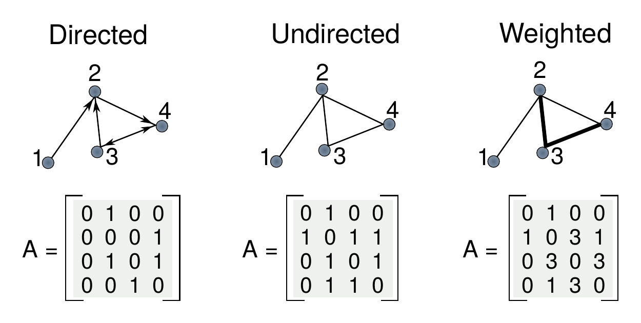
Figure 2.1: Schematic representation of directed, undirected and weighted networks. In directed graphs a relationship from \(i\) to \(j\) does not imply that the reciprocal is true, hence the adjacency matrix is not symmetric. In undirected graphs all relationships are reciprocal, making the matrix symmetric. In weighted graphs links have associated weights which can represent various quantities such as the strength or duration of the interaction.

The fundamental mathematical representation of a network is the adjacency matrix, \(A\). Given a graph composed by \(N\) nodes, its adjacency matrix is a square matrix of size \(N\times N\) in which \(a_{ij}=0\) if there is no relationship between nodes \(i\) and \(j\) and \(a_{ij}\neq 0\) otherwise. Depending on the values allowed for \(a_{ij}\) we can define several types of graphs. The most common one is the undirected binary graph, undirected graph or, simply, graph, in which the matrix is symmetric and \(a_{ij}\) can only take binary values. If we relax the symmetry condition we obtain a directed graph, in which a relationship from node \(i\) to node \(j\) does not imply the existence of a relationship from \(j\) to \(i\). Even more, if we allow \(a_{ij}\) to take any positive value, we obtain a weighted graph. In these networks links have an associated weight that represents the relative strength of the interaction. A schematic representation of these three types of networks is shown in figure 2.1. During this thesis we will explore the three of them, although the undirected graph is admittedly the most common one.

Although the adjacency matrix completely describes a network, it is rather difficult for humans to comprehend the structure of the network by just looking at its adjacency matrix. For this reason, it is common practice to define mathematical measures that capture interesting features of network structure quantitatively. In the following section we will describe the ones that will be used all over the thesis.

2.1.1 Topological properties of networks

The most basic microscopic property is the degree of the nodes, which represents the number of links it has. For a network of \(N\) nodes the degree can be written in terms of the adjacency matrix as

\[\begin{equation} k_i = \sum_{j=1}^N a_{ij}\,. \tag{2.1} \end{equation}\]

This quantity plays a key role in many networks. In fact, networks can be classified according to their degree distribution, \(P(k\)), which provides the probability that a randomly selected node in the network has degree \(k\). It has been observed that the precise functional form of \(P(k)\) determines many network phenomena in a wide array of systems. Besides, with this distribution, it is possible to obtain other important quantities such as the average degree of a network

\[\begin{equation} \langle k \rangle = \sum_{k=0}^\infty k P(k) \tag{2.2} \end{equation}\]

In directed networks, (2.1) is slightly different as the network is not symmetric. Thus, we have to define the in-degree as the number of incoming links to a node and the out-degree as the number of outgoing links,

\[\begin{equation} k_i^\text{in} = \sum_{j=1}^N a_{ij} \,, \quad \quad k_i^\text{out} = \sum_{j=1}^N a_{ji} \tag{2.3} \end{equation}\]

In the case of weighted networks, it is common to denote with the binary quantity \(a_{ij}\) the existence of a link, while the weight is encoded in the variable \(w_{ij}\). This way, it is possible to use the same definition for the degree (2.1) and, similarly, define the strength of a node as

\[\begin{equation} s_i = \sum_{j=1}^N w_{ij} \, . \tag{2.4} \end{equation}\]

In a similar fashion, one can define as many observables as desired, some of which will be more important than others depending on the system under consideration. In particular, a lot of effort has been devoted to the concept of centrality in networks, which tries to answer the question of which are the most important nodes in a network. There are multiple ways of defining the centrality of a node and the best one usually depends on the specific system that is being analyzed. For instance, the degree of a node by itself can be considered as a measure of its importance. However, as we shall see, our interest in this thesis lays on the role nodes play in transportation networks. Hence, for us, it is more interesting to know which nodes are indispensable for the correct operation of the network rather than which are the most popular. For instance, one can think of two large parts of a city divided by a river with one bridge. It is clear than in said situation the bridge holds a key position in the system, as if there was a problem there, both parts of the city would become disconnected. A quantity that can capture this information is the betweenness.

To understand betweenness we first need to talk about paths. A path is a route that runs along the links of a network without stepping twice over the same link. We define the shortest path between nodes \(i\) and \(j\) as the path between them with the fewest number of links. Note that if we had a weighted network representing some spatial system, with the real spatial distance acting as weight, this is equivalent to simply look for the route between two nodes that minimizes the total distance traveled.

Denoting by \(\sigma^i_{rs}\) the number of shortest paths between nodes \(r\) and \(s\) that pass through \(i\), the betweenness of node \(i\) can be defined as

\[\begin{equation} b_{i} = \frac{2}{(N-1)(N-2)} \sum_{r\neq i}\sum_{s \neq i} \frac{\sigma_{rs}^i}{\sigma_{rs}}\,, \tag{2.5} \end{equation}\]

that is, the fraction of all shortest paths in the system that include node \(i\) without starting or ending in it. The leading factor is just a normalization constant so that the betweenness of networks of different sizes can be compared.

2.1.2 Important degree distributions

As previously mentioned, the degree distribution of a network can determine many of its properties. Although any probability distribution can be used as a degree distribution, there are two prototypical distributions to which this section will be devoted: the Poisson distribution and the power-law distribution.

The Poisson distribution attains its importance from being the distribution that arises naturally in the random graph model. In general, a random graph is a model network in which the values of certain properties are fixed, but it is in other respects random. One can think of many properties that could be settled, but undoubtedly the simplest choice is to establish the number of nodes \(N\) and the number of links \(L\). Such model is known as Erdős-Rényi model} (honoring the contributions of Paul Erdős and Alfréd Rényi in the study of the model [76]), ER graph, Poisson random graph* or, simply, "the’’ random graph. Henceforth, we will refer to this model as ER.

In the ER model the only two elements that are fixed are the number of nodes, \(N\), and the number of links, \(L\). Hence, this model does not define a single network but rather a whole collection of networks, or ensemble, that are compatible with those constraints. Indeed, as there are \(\binom{N}{2}\) ways of selecting pairs of nodes, there are \(\binom{\binom{N}{2}}{L}\) ways of placing the \(L\) links, or different graphs. The probability of selecting any of those graphs will be given by

\[\begin{equation} P(G) = \frac{1}{\dbinom{\binom{N}{2}}{L}}\,. \tag{2.6} \end{equation}\]

Although this is the original formulation of the model, nowadays it is more common to use a definition that is completely equivalent for large \(N\). Specifically, one defines \(p\) as the probability of including any possible link, independently from the rest of links. Therefore, for instance, the average degree in both formulations would be \[\begin{equation} \langle k \rangle = \frac{2L}{N} = p(N-1) \,. \tag{2.7} \end{equation}\]

To obtain the degree distribution of this model we need to consider that a given node in the network will be connected with probability \(p\) to each of the \(N-1\) other nodes. Thus the probability of being connected to \(k\) nodes and not to the rest of them is \(p^k(1-p)^{N-1-k}\). As there are \(\binom{N-1}{k}\) ways to choose \(k\) nodes, the probability of being connected to \(k\) nodes is

\[\begin{equation} P(k) = \binom{N-1}{k} p^k (1-p)^{N-1-k}\,, \tag{2.8} \end{equation}\]

which is a binomial distribution. Yet, in many cases we are interested in the properties of large networks, so that \(N\) can be assumed to be large. In the large-\(N\) limit equation (2.8) tends to a Poisson distribution,

\[\begin{equation} P(k) = \frac{(pN)^k e^{-pN}}{k!} \approx \frac{\langle k \rangle^k e^{-\langle k \rangle}}{k!}\,. \tag{2.9} \end{equation}\]

Due to its simplicity, this model is often used as the basic benchmark to determine if a real network has non trivial topological structures. Yet, most real networks do not resemble an ER graph at all. Actually, the most common distribution of real networks is a power law distribution. A power law distribution can be expressed as

\[\begin{equation} P(k) = C k^{-\gamma}\, \tag{2.10} \end{equation}\]

where \(C\) is the normalization constant that ensures that the probability is correctly defined. Networks with a degree sequence that follows a power law distribution are known as scale-free (SF) networks.

The term scale-free comes from the fact that the moments of the power-law distribution,

\[\begin{equation} \langle k^n \rangle = \int_{k_\text{min}}^{k_\text{max}} k^n P(k) \text{d}k = C \frac{k_\text{max}^{n-\gamma+1}-k_\text{min}^{n-\gamma+1}}{n-\gamma + 1}\,, \tag{2.11} \end{equation}\]

diverge under certain conditions. In particular, if \(2<\gamma<3\) and \(k_\text{max} \sim \sqrt{N} \rightarrow \infty\) the first moment is finite, but the second moment diverges. Interestingly, most networks following a power law distribution have an exponent between 2 and 3. Hence, the fluctuations around \(\langle k \rangle\) are so large that a given node could have a very tiny degree or an arbitrarily large one. In other words, there is no ``scale’’ in the network. In contrast, if the degree distribution is Poisson, a node is expected to have degree in the range \(k = \langle k \rangle \pm \langle k \rangle^{1/2}\). Thus, in those cases, \(\langle k \rangle\) serves as the scale of the network.

This property of both degree distributions gives rise also to another terminology. Sometimes ER networks are said to be homogeneous while SF networks are called heterogeneous. As we shall see, this heterogeneity is the origin of some of the most interesting phenomena in network science.

2.1.3 Multilayer graphs

The methodology presented so far has always considered that all the links in a network represent the same kind of relationship. But, for instance, if we think of a social interaction network, it is clear that relationships can be of very diverse nature. Thus, given a diverse system, we can classify its interactions into groups according to their characteristics. This classification yields a set of networks, one for each interaction, related to each other. The way in which these networks are connected to one another, the entities their nodes represent and the way their relationships are represented, produce a new set of networks that goes beyond the concept of simple graphs. We call these structures multilayer networks [77]. When talking about multilayer networks, one often refers to the graphs presented so far as single-layer networks or monoplex networks.

In multilayer networks, we have an extra ingredient apart from nodes and links, layers, which contain the networks defined by each interaction type as discussed above. In its most general form, a multilayer network is composed by nodes that can be connected to other nodes in the same layer or to nodes in different layers. Then, depending on the specific system under consideration, it is possible to have several types of multilayer networks. For instance, if nodes represent the same entity in all layers we say that we have a multiplex network (although the definition of multiplex network is slightly more general, as the main requirement is that all nodes have their counterparts in other layers, regardless of them representing the same entity or not). A paradigmatic example of such objects are social networks, where nodes represent individuals participating in social interactions. If an individual has relationships in two different contexts, we will find the node representing that person in two layers.

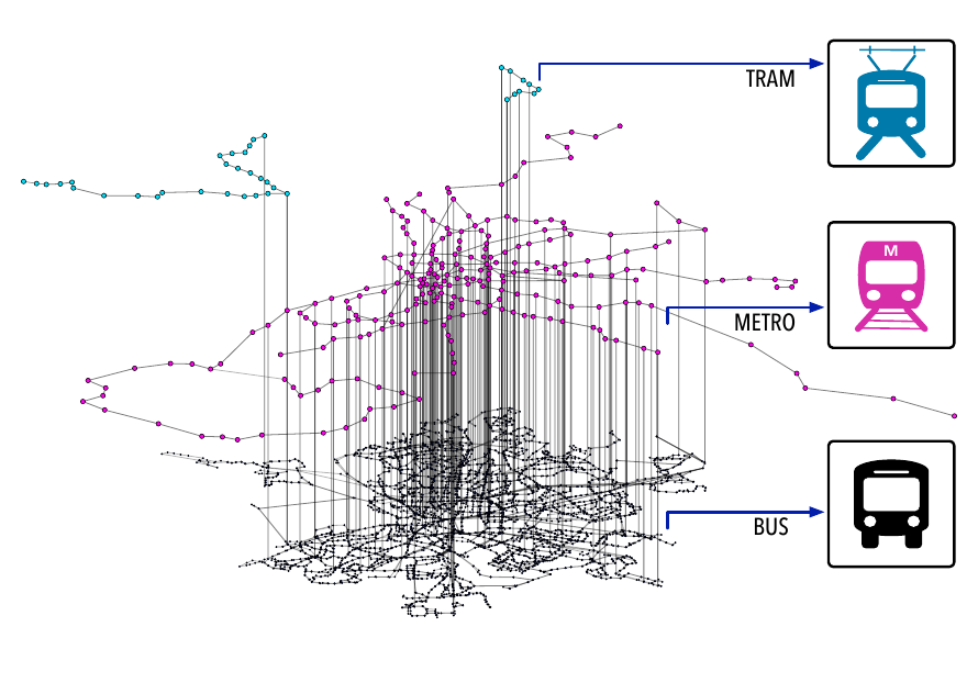
Figure 2.2: Multilayer representation of Madrid’s public transportation system. Nodes in the bottom layer (black) represent bus stops, with a link between two nodes if at least one bus line connects them. In the middle layer (pink) nodes are metro stops and links their corresponding metro lines. Lastly, the top layer (blue) is composed by tram stops and their connections. Nodes in different layers are connected if they are within 100 meters.

Another system that can be effectively represented using multilayer networks is the public transportation system of a city. To illustrate this, in figure 2.2 we show the multilayer representation of Madrid’s public transportation network. In this case, each transportation mode is encoded in a distinct layer, with nodes representing bus, metro and tram stops. To take into account the possibility of commuting, e.g., taking first the metro and later a bus, a link connecting nodes in different layers is set if they are within a reasonable walking distance. Thus, in this case, nodes do not represent exactly the same entity (although one could argue that they represent the same physical location) and links across layers have a clear physical meaning.

There are two main approaches to encode multilayer networks in a mathematical object: tensors and supra-adjacency matrices [78]. For simplicity, we will only present the latter approach, as it is straightforward to extend the notions of classical graph theory into multilayer graphs this way.

Suppose that we have two single-layer networks as depicted in figure 2.3A, encoded in their respective adjacency matrices, \(A_1\) and \(A_2\). These matrices contain information about the links that are set inside each layer, the intra-layer links. Now, suppose that these two networks are not isolated but are allowed to interact, or represent different parts of the same system. In such scenario we can build a coupling matrix, \(C\), containing the links that connect nodes in different layers, the inter-layer links. These matrices allow us to define the supra-adjacency matrix as

\[\begin{equation} A = \oplus_\alpha A_\alpha + C\,, \tag{2.12} \end{equation}\]

where \(\alpha\) runs over the set of layers. This matrix is shown in figure 2.3B, where both layers interact via nodes \(1-4\) and \(2-5\).

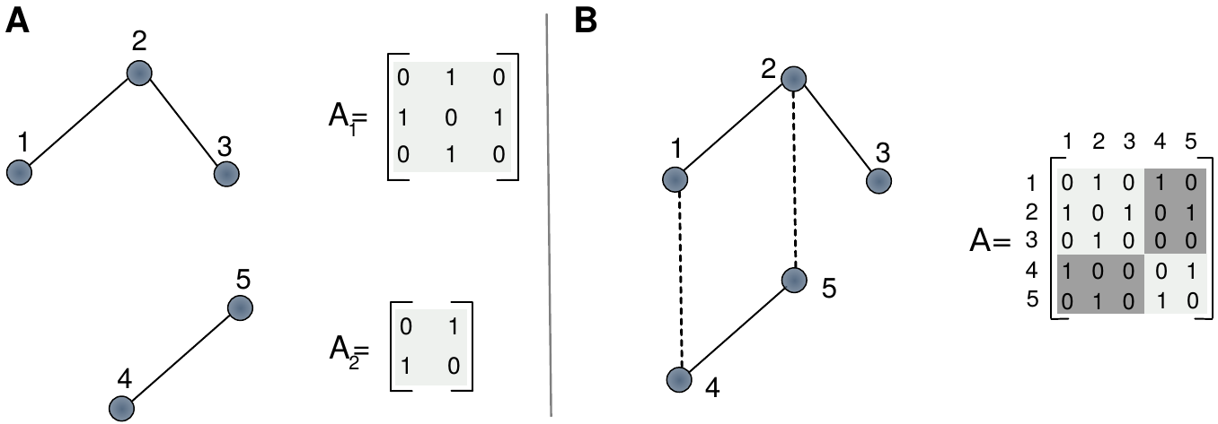
Figure 2.3: Schematic representation of multilayer networks. A) Two independent graphs with their respective adjacency matrices. B) A multilayer network made of both networks with its supra-adjacency matrix.

The same way we defined in monoplex networks the degree of a node as the sum of its links, in multilayer networks the degree of node \(i\) in layer \(\alpha\) reads

\[\begin{equation} k_i^\alpha = \sum_j a_{ij}^\alpha\,. \tag{2.13} \end{equation}\]

Note that this implies that the degree of a node is no longer a scalar but a vector \(k_i = (k_i^1,\ldots,k_i^L)\). Nevertheless, we can recover the equivalent quantity of degree in monoplex networks denominated degree overlap as

\[\begin{equation} o_i = \sum_\alpha k_i^\alpha\,. \tag{2.14} \end{equation}\]

A similar procedure can be followed to extend the notion of strength in the case of weighted multilayer networks.

To conclude this section, let us point out the existence of measures that only exist in multilayer networks, without single-layer counterparts. For instance, the interdependence of node \(i\) is defined as

\[\begin{equation} \lambda_i = \sum_{i\neq j} \frac{\psi_{ij}}{\sigma_{ij}}\,, \tag{2.15} \end{equation}\]

where \(\sigma_{ij}\) is the total number of shortest paths between nodes \(i\) and \(j\) and \(\psi_{ij}\) is the number of shortest paths between those nodes that make use of links in two or more layers. Hence, the interdependence measures how dependent a node is on the multiplex structure in terms of reachability. To understand this property we can have a look again at figure 2.2. In that network, it is clear that to reach most nodes from any tram stop it is required to go through more than one layer, making tram stops quite interdependent. Conversely, it is possible to reach almost all nodes from a bus stop without having to go through other layers. This example highlights that sometimes individual nodes are not that important, as the layer they are in already determines some of their properties. In this particular example, it is then useful to extend the definition of interdependence from nodes to layers to account for the importance of a given layer in the whole system [79].

2.2 The problem of null models

For some systems, networks naturally provide the skeleton on which dynamical processes can be studied, allowing us to predict the outcome of such processes under different conditions. However, in Jaynes’ words [30], prediction is only one of the functions of statistical mechanics. Equally important is the problem of interpretation; given certain observed behavior of a system, what conclusions can we draw as to the microscopic causes of that behavior?

To this aim, one of the main focus of network science is to determine the empirical properties of a network that provide the maximum amount of information about the network itself or about the dynamical processes taking place in the system that the network represents [80]. In order to do so, a standard approach is to create a null model of the network that will act as a benchmark model. Then, it is possible to identify which properties deviate from what is “expected” in rigorous statistical terms. This, in turn, has several implications. First, it highlights which properties might bear important information about the system dynamics. Similarly, it can be used to detect the hidden mechanisms behind the formation of the network structure, by pointing out the properties that the model was not able to capture. Furthermore, it can be used to elucidate which characteristics of the network are truly important and which ones are just a consequence of lower-order attributes.

Indeed, suppose that we measure two properties of a real network, \(X\) and \(Y\). Then, we build a null model of the network using only information about \(X\). If most networks in the ensemble of randomized graphs exhibit property \(Y\), we can state that \(X\) explains \(Y\) and thus any attempt of analyzing \(Y\) without considering \(X\) is futile. For instance, many real networks exhibit what is known as the small-world property, meaning that the average length of shortest paths in the network scales as \(l \propto \ln(N)\) rather than with the number of nodes [56]. Yet, while in sparse networks like social networks it is a genuine feature of the system, in highly dense networks, such as the interarial cortical network in the primate brain where 66% of links that could exist do exist, it is just a consequence of the huge amount of links present in the network [81].

The previous example shows that sometimes \(Y\) can be just a consequence of a particular value of \(X\). However, it is also possible to find properties \(Y\) that are always a direct byproduct of \(X\), rendering them redundant. For instance, it has been observed that many ecological networks of mutualistic interactions between animals and plants are nested, that is, that interactions of a given node are a subset of the interactions of all nodes with larger degree. Yet, despite being a widely used metric in the field of ecology, it was recently demonstrated that the degree sequence of the network completely determines the nestedness of the system. Note that to calculate the nestedness of a network it is necessary to know the whole adjacency matrix, while the degree sequence is just the number of non zero entries per row. Hence, the nested pattern is not more informative of the behavior of real systems than their degree sequence alone. In other words, attempting to explain why an ecological system exhibits a given value of nestedness is pointless, as the focus should be on elucidating the mechanisms that give rise to a particular degree sequence [82].

The applications of null models go far beyond the determination of which properties of the network are important. For instance, when not all the information of a system is available, they can be used to infer missing information or to devise adequate sampling procedures to reduce it [83], [84]. Another interesting and open problem is that network data may contain errors inherent to any experimental measurement. Null models can then be used to estimate the errors in the data and even to correct them [73].

However, as with any hypothesis test, the choice of the null model can directly affect the conclusions. Hence, care must be taken when deciding which one is the best suited for the system under consideration. There are two possible approaches to create null models of networks. The first one consists in building networks based on heuristic rules that are compatible with the specific characteristics of the real system. A classical example is that of gravitational models, widely used in economical and spatial systems way before the birth of network science [85], [86], in which an interaction between two entities depends inversely on their distance and proportionally to their “mass”, be it products or population. This method can also be used to shed some light on the mechanisms driving the evolution of networks, rather than just as a tool for generating randomized networks. For instance, the Barabási-Albert model was proposed as a plausible explanation of the emergence of scale-free networks. This model is based on, at each iteration, adding a new node into the network and linking it to \(m\) existing nodes, chosen with probability proportional to their degree. This preferential attachment naturally leads to networks exhibiting the scale-free property [87].

These types of models, however, can be either too domain specific or require several refinements to give quantitatively accurate predictions [60]. Hence, frequently, a better approach is to identify a set of characteristic properties of the real network and then build a collection or ensemble of networks with those same properties but otherwise maximally random. Despite its conceptual simplicity, this approach has several subtleties that have to be properly handled, something that, as we shall see, is not systematically done. Additionally, we can distinguish two different families of models within this approach: the microcanonical, in which properties are exactly fixed, and the canonical, in which properties are preserved on average.

2.2.1 Microcanonical models

Microcanonical approaches are based on generating randomized variants of real networks in such a way that some properties are identical to the empirical ones. However, although their simplicity makes them quite appealing, most of them suffer from problems such as bias, lack of ergodicity or mathematical intractability [88]. Yet, they are widely used, even if not always correctly.

The simplest microcanonical ensemble of graphs that can be built is based on fixing the total number of links, \(L\), and otherwise keeping the graphs completely random. This, as we show in section 2.1.2, defines the ER model. The problem of this model is that it is overly simplistic and real networks often exhibit much richer structures. Thus, a more common approach is to fix the degree of the nodes, also known as degree-preserving randomization or configuration model. To see why this is a good option, note that \(L\) can be obtained by adding up the whole degree sequence. Hence, as discussed previously, if we were able to reproduce the degree distribution of a network by just fixing \(L\), it would not convey any valuable information about the network. However, we showed in section 2.1.2 that the degree distribution in the ER model is Poisson, whereas in most real networks it follows a power law distribution. In other words, the degree sequence often provides much more information about the system than just the number of links.

To build graphs with a fixed degree sequence, two different approaches can be followed: a bottom-up and a top-down approach. The work by Maslov et al. in 2002 on protein and gene networks [89] is often cited as one of the earliest examples of degree-preserving randomization. Another common reference (for instance, in the wikipedia entry on degree-preserving randomization [90]), is the work by Rao et al. in 1996 [91] on generating random \((0,1)\)-matrices with given marginals. Yet, both methods fall into the category of top-down approaches but, historically, bottom-up approaches were introduced much earlier. In fact, this is one of those methods that have been independently rediscovered several times in different fields, usually with different terminology as well [92]. For instance, in sociology this approach can be traced back to 1938 [93] and in ecology to 1979 [94].

For historical reasons, let us begin with the bottom-up approach. The basic idea is to attach to each node as many “link stubs” as its degree in the original network. Then, pairs of stubs are randomly matched, generating graphs that preserve the original degree sequence. In the context of graph theory stub matching was introduced by Bollobás in 1980 [95]. He called each of the graphs extracted from the ensemble a “configuration”, from which the term configuration model emerges, even though nowadays it is used to refer to any model that preserves the degree sequence of the network. Note also that for this approach it is not necessary to have knowledge of the whole adjacency matrix, as only the total addition of its rows and columns are needed. Thus, this procedure is suitable also to create graphs based on a degree sequence sampled from any degree distribution, and not only to randomize existing networks.

Unfortunately, stub matching presents several drawbacks. First, even if the original network is simple (and most real networks are), this method naturally allows both multilinks and self-loops. It is sometimes argued that this is not a problem as their number tends to zero as the size of the graphs grows [73]. However, this is not true in general for scale-free networks, which are the most common ones. Even more, real networks are always finite, and in some fields such as ecology rather small, making this method unsuitable for their randomization. A widely proposed solution is to reject multilinks or self-loops [60], [96], but this, again, has numerous issues. Indeed, when most stubs are already matched, it is possible that the remaining ones cannot be matched, as there might be already links between the nodes with remaining open stubs. Furthermore, this procedure no longer samples uniformly the space of graphs, introducing some biases. In the famous work by Catanzaro et al. on the generation of scale-free networks [97], it was shown that this bias can be solved by imposing the maximum degree in the network to be \(k_\text{max} \leq N^{1/2}\). Although this might be a suitable approach for creating random networks from scratch, it is clearly not valid for randomizing real networks, in which the maximum degree often exceeds such limit (see figure 2.4A). Several other modifications have been proposed to fix stub matching for simple networks, but there is not a clear solution that always works [92].

Figure 2.4: Topological properties of 1326 real networks. These networks represent the whole Koblenz Network Collection spanning over 24 different types of systems, from online to infrastructure or trophic networks [98]. In A the maximum degree of each network as a function of its number of nodes is shown. The line represents the structural cutoff \(k_{max} = N^{1/2}\) of the uncorrelated configuration model [97]. In B the maximum degree is plotted against the total degree of the network (note that \(k_{tot} = 2L\)). The line represents the structural cutoff \(k_{max} = (2L)^{1/2}\) above which equation (ref:eq:chap2-null-cutoff) is not valid.

Conversely, the top-down approach starts with the full adjacency matrix and randomizes it. In this case, the idea is to take existing links and randomly change which nodes they are attached to. For this reason, this procedure is also known as rewiring. The straightforward approach would be to simply randomize the entries of the adjacency matrix, but this procedure would yield the same results as the ER model with fixed number of links [75]. A better idea is, thus, to take two pairs of connected nodes and swap their links, so that the degree sequence of the network is exactly preserved. Howbeit, this procedure is neither free of caveats. For instance, the number of necessary rewires to effectively randomize the network is unknown a priori, spaning several orders of magnitude depending on the network under consideration [99]. Even more important, swaps are usually proposed to be such that given two pairs of connected nodes, \(\{a,b\},\{c,d\}\), the rewiring results in \(\{a,d\},\{b,c\}\) [96]. However, note that the rewiring \(\{a,c\},\{b,d\}\) is perfectly valid too [100], but it is often concealed because if the two randomly selected links are \(\{a,b\},\{a,c\}\), this last swap would introduce a self-loop in the system. Similarly, multilinks can also appear in the graph, unless we strictly forbid them. Yet, if this is naively done biases will be introduced in the sampling procedure, although there are advanced techniques that can be applied to solve these problems in some cases [92], [100].

Yet, it is stricking that even though the biases of the naive link swapping have been known for years [101], this method is still widely used today. One could even argue that it is actually the most common one, as it is recommended in recent books [75], [96] and some of the most widely used software packages for studying networks do not take into account the necessary corrections in their routines [102]. In particular, it was shown [104] that naive rewiring sampling is only uniform as long as

\[\begin{equation} \langle k^2\rangle k_\text{max} / \langle k \rangle^2 \ll N\,. \tag{2.16} \end{equation}\]

But we know that in scale-free networks \(\langle k^2 \rangle\) diverges, making this approach ill-suited for strongly heterogeneous networks, the most common ones.

It is clear then, that even if the main ideas of microcanonical models are easy to understand, properly implementing them is not as straightforward as it may seem and multiple subtleties have to be taken into account. Furthermore, so far we have only discussed about binary networks as extending these concepts to weighted graphs is not an easy task either. For instance, one could propose that when swapping links its weight should be attached to it, as if we were directly randomizing the adjacency matrix. Another possible choice would be to only shuffle weights over links, keeping the latter fixed to their nodes. Or even creating stubs with fixed weights and only matching those with equal values, and many more [105]. Obviously, each choice might have its own advantages and drawbacks, but there is no doubt that using such null models should rise more questions than answers about the system.

2.2.2 Canonical models

In canonical models, rather than generating randomized networks, the main objective is to determine mathematical expressions for the expected topological properties as a function of the imposed constraints. Nevertheless, sampling random graphs from canonical ensembles is not only possible but often necessary, as we will see in section 2.5.1.

Focusing on binary graphs [88], since any topological property \(X\) is a function of the adjacency matrix \(A\), the goal is to determine the probability of occurrence for each graph, \(P(A)\). This allows the computation of the expected value of \(X\) as \(\sum_A P(A) X(A)\) without resorting to sampling adjacency matrices. More importantly, in canonical ensembles where the properties that we want to preserve are local, \(P(A)\) factorizes to a product over the probability \(p_{ij}\) that nodes \(i\) and \(j\) are connected.

For instance, if we choose \(p_{ij} = p \quad \forall i,j\) we obtain the canonical version of the ER model, which in the limit \(N\rightarrow \infty\) is equivalent to the microcanonical setup in which the number of links is fixed. Note that in the former setting \(p_{ij} = p\) is the same as fixing the number of links to be \(p\binom{N}{2}\).

If, instead, one wishes to preserve the degree sequence of the network, the most popular choice of \(p_{ij}\) is

\[\begin{equation} p_{ij} = \frac{k_i k_j}{k_\text{tot}} = \frac{k_i k_j}{2L} \tag{2.17} \end{equation}\]

which can be clearly related to the problem of stub matching described in section 2.2.1. Despite its popularity and widespread use, it is important to note - although often disregarded - that this expression is only valid for uncorrelated networks, i.e., as long as the largest degree in the network does not exceed the so-called structural cut-off [106],

\[\begin{equation} k_\text{max} \leq \sqrt{k_\text{tot}} = \sqrt{2L}\,. \tag{2.18} \end{equation}\]

But, as we can see in figure 2.4B, most networks do not fulfill this condition. Hence, if we were to use equation (2.17) to determine if a given property of the network can be explained just by its degree sequence, we would be making a mistake as the own degree sequence already has a property that our model is not capturing. Thus, an expression that correctly captures degree correlations should be used instead. This is not to say that the reasons why correlations or, similarly, large degrees appear in the network are not important. On the contrary, they are, but if they are not added into the null model we will not be able to discern if a given feature of the network is truly meaningful or just a byproduct of the unavoidable correlations. In addition to all of this, equation (2.17) is not a correct probability as one can easily think of toy models in which \(p_{ij}>1\).

The problems induced by highly heterogeneous networks, the most common type of real networks, are clearly challenging most null models, both microcanonical and canonical. In what follows, we will introduce an approach that can solve all these problems and provide a unified approach to sample graph ensembles with local constraints in an unbiased way, the exponential random graph model.

2.3 Exponential random graphs

Suppose that we want to build a simple, binary and undirected graph based only on two macroscopic properties: its number of nodes, \(N\), and its number of links, \(L\). As in the classical problems of statistical mechanics, the number of microstates - graphs - that are compatible with those macroscopic quantities is quite large. Indeed, as we are considering simple graphs, the number of microstates can be obtained from counting the number of ways in which we can select \(L\) elements from the set of node pairs, \(C_2^N\). As such,

\[\begin{equation} \begin{split} \Omega & = C^{C^N_2}_L =\dbinom{\binom{N}{2}}{L}= \binom{\frac{N(N-1)}{2}}{L} = \frac{\frac{N(N-1)}{2}!}{L!\left(\frac{N(N-1)}{2}-L\right)!} \\ & \approx \exp\left[L\log\left(\frac{N(N-1)}{2L}-1\right) - \frac{N(N-1)}{2}\log\left(1-\frac{2L}{N(N-1)}\right)\right] \,, \end{split} \tag{2.19} \end{equation}\] where we have used Stirling’s approximation to the factorials.

To illustrate, we can take the example of a seemingly small network, the neural network of the nematode Caenorhabditis elegans (or simply C. elegans) which was the first - and so far, only - animal to have the whole nervous system (almost) completely characterized [107]. This little worm, of about \(1\) mm in length, possesses 302 neurons and about 5600 synapses (considering for simplicity both chemical and electrical synapses undirected) as measured by Brenner et al. in 1986 after 15 years of work [108] (the most recent measurements have increased this number slightly above 6000 [109]). Even though small in comparison with the neural system of organisms such as the fruit fly, with over \(10^5\) neurons, or the human, with over \(10^{10}\) neurons, the total amount of compatible microstates of this system is

\[\begin{equation} \Omega = \dbinom{\binom{302}{2}}{5600} \approx e^{16966} \sim 10^{7368} \,. \tag{2.20} \end{equation}\]

No wonder, then, that this network is still being intensely studied today. To asses even further the importance of this little network, suffice to say that the work by Brenner et al. not only was the starting point of the field of connectomics, but it also created a whole field of research around this organism from which three Nobel Prizes honoring eight scientists have been awarded to date [107].

This example clearly shows that a huge amount of different graphs can give rise to the same macroscopic properties. However, as described in section 2.2, this can actually be a powerful tool to asses what are the main topological characteristics of a network, or which ones are just a consequence of others. The problem is, then, on how to build an ensemble of networks using only partial information of the real one.

Fortunately, this question was already answered by Jaynes in the context of statistical mechanics using the results provided by information theory [30]. Indeed, given a certain quantity \(G\) which can take the discrete values \(G_i (i=1,\ldots,n)\) and the expectation value of the function \(f(G)\),

\[\begin{equation} \langle f(G) \rangle = \sum_{i=1}^n p_i f(G_i) \,, \tag{2.21} \end{equation}\]

where \(p_i\) is the probability of finding \(G_i\) in the ensemble. The only way to set these probabilities without any bias, while agreeing with the given information, is to maximize Shannon’s entropy,

\[\begin{equation} S = -\sum_{i=1}^n p_i \ln p_i \,, \tag{2.22} \end{equation}\]

subject to the appropriate constraints derived from the information. Applied to statistical mechanics, this meant that the old Laplacian principle of insufficient reason according to which, in absence of evidence, the same probability should be assigned to each possible event was not needed anymore (although it is still regarded as one of the basic postulates of statistical mechanics [110], [111]). Instead, the same proposition could be read in positive as maximizing the uncertainty in the probability subject to whatever is known, thus removing the apparent arbitrariness of the principle of insufficient reason. It is trivial to see that if there are not any constraints the maximum entropy is attained for the uniform probability distribution.

Back into the context of networks, following Park and Newman [54], suppose that the information we have is a collection of graph observables \({X_i}\), \(i=1,\ldots,r\) from which we have an estimate of their expectation value, \(\langle X_i \rangle\), measured over a real network. Let \(G\) be a graph in the set of all simple graphs of \(N\) nodes, \(\mathcal{G}\), and let \(P(G)\) be the probability of finding that graph in the ensemble. According to our previous discussion, the most unbiased method to assign values to said probabilities given the available information is to maximize the entropy

\[\begin{equation} S = - \sum_{G\in\mathcal{G}} P(G) \ln P(G) \tag{2.23} \end{equation}\]

subject to the constraints

\[\begin{equation} \sum_{G\in\mathcal{G}} P(G) X_i(G) = \langle X_i \rangle \tag{2.24} \end{equation}\]

plus the normalization condition

\[\begin{equation} \sum_{G\in\mathcal{G}} P(G) = 1\,, \tag{2.25} \end{equation}\]

where \(X_i(G)\) denotes the value of the observable \(X_i\) in graph \(G\).

To impose these constraints in the maximization process we can introduce the Lagrange multipliers \(\alpha\), \({\theta_i}\), so that

\[\begin{equation} \frac{\partial}{\partial P(G)} \left[S+\alpha\left(1-\sum_{G\in\mathcal{G}}P(G)\right)+\sum_{i=1}^r \theta_i \left(\langle X_i \rangle - \sum_{G\in\mathcal{G}} P(G) X_i(G)\right)\right] = 0 \tag{2.26} \end{equation}\]

for all graphs \(G\). This gives

\[\begin{equation} \ln P(G) + 1 + \alpha + \sum_{i=1}^r \theta_i X_i(G) = 0 \,, \tag{2.27} \end{equation}\]

or equivalently

\[\begin{equation} P(G) = e^{-(1+\alpha+\sum_{i=1}^r \theta_i X_i(G))} \,. \tag{2.28} \end{equation}\]

Now, inserting this last equation into (2.25) we can define the variable \(Z\) as

\[\begin{equation} \begin{split} \sum_{G\in\mathcal{G}} P(G) & = \sum_{G\in\mathcal{G}} e^{-(1+\alpha+\sum_{i=1}^r \theta_i X_i(G))} = 1 \\ \Rightarrow & Z \equiv \sum_{G\in\mathcal{G}} e^{-\sum_{i=1}^r \theta_i X_i(G)} = e^{1+\alpha}\,. \end{split} \tag{2.29} \end{equation}\]

Hence, the exponential random graph model is completely defined by

\[\begin{equation} P(G) = \frac{e^{-H(G)}}{Z}\,, \tag{2.30} \end{equation}\]

where \(H(G) = \sum_{i=1}^r \theta_i X_i(G)\) is the graph Hamiltonian and \(Z=\sum_{G\in\mathcal{G}} e^{-H(G)}\) is the partition function. Note that this expression is equivalent to the probability distribution for the canonical ensemble of statistical physics, which can actually be derived using the same procedure considering an isolated system in thermal equilibrium with the energy as observable [112]. Thus, it represents the graph analog of the Boltzmann distribution. Actually, the classical parametrization of the Boltzmann distribution, i.e., using \(\beta\) instead of \(\theta\), gave the name to the \(\beta\)-model, which is the exponential random graph model in the particular case of undirected graphs [113].

Using (2.30) it is then possible to measure the expected value of any graph property \(Y\) over the ensemble,

\[\begin{equation} \langle Y \rangle = \sum_{G\in\mathcal{G}} P(G) Y(G)\, , \tag{2.31} \end{equation}\]

obtaining the best estimate of the unknown quantity \(Y\) given the set of known quantities \({X_i}\).

Before going any further, it might be enlightening to see a simple example. Suppose that we only know the average number of links, \(\langle m \rangle\), of our network. In that case the Hamiltonian is just

\[\begin{equation} H(G) = \theta m(G) \,. \tag{2.32} \end{equation}\]

Let \(A\) be the adjacency matrix of graph \(G\) with \(N\times N\) nodes and elements \(a_{ij} = {0,1}\). Then, the number of links is \(m=\sum_{i<j} a_{ij}\) and the partition function is

\[\begin{equation} \begin{split} Z & = \sum_{G\in\mathcal{G}} e^{-H(\theta)} = \sum_{\{a_{ij}\}} e^{-\theta \sum_{i<j} a_{ij}} = \sum_{\{a_{ij}\}} \prod_{i<j} e^{-\theta a_{ij}} \\ & = \prod_{i<j} \sum_{a_{ij}=0}^1 e^{-\theta a_{ij}} = \prod_{i<j}(1+e^{-\theta}) = [1+e^{-\theta}]^{\binom{N}{2}} \end{split} \tag{2.33} \end{equation}\]

so that

\[\begin{equation} P(G) = \frac{e^{-H(\theta)}}{Z} = \frac{e^{-\theta m}}{[1+e^{-\theta}]^{\binom{N}{2}}} = p^m (1-p)^{{\binom{N}{2}}-m}\,, \tag{2.34} \end{equation}\]

where we have defined \(p\equiv (e^\theta + 1)^{-1}\).

Recalling section 2.1 we can clearly see that equation (2.34) is just the well known Erdős and Rényi graph, or random graph. Thus, it seems that we have achieved our objectives, building a graph that satisfies our constraints but otherwise completely random, hence its name.

As an example of how to calculate expected values of graphs over this ensemble, we show how to obtain the expected degree, which we know should be equal to \(p(N-1)\) (equation (2.7)),

\[\begin{equation} \begin{split} \langle k \rangle & = \frac{2 \langle m \rangle }{N} = \frac{2}{N} \frac{1}{Z} \sum_{G\in\mathcal{G}} m e^{-\theta m} = -\frac{2}{N}\frac{1}{Z}\frac{\partial Z}{\partial \theta} = \frac{2}{N}\binom{N}{2}\frac{1}{e^\theta + 1} \\ & = \frac{2}{N} \binom{N}{2} p = \frac{2}{N} \frac{N(N-1)}{2} p = (N-1)p\,. \end{split} \tag{2.35} \end{equation}\]

2.4 Randomizing real networks

We have seen that equation (2.31) allows us to calculate expected values of graph observables over an ensemble of maximally random graphs restricted to the information we have of the system. However, in some occasions the observables we are interested in might not have an analytic closed-form solution. Or we might be interested in the effect of a given dynamical process on the network and we would like to know if in networks with equivalent macroscopic properties the outcomes would be similar. In those cases, the only thing we can do is to directly sample a large amount of networks from the constructed ensemble and measure the desired topological properties or implement the dynamical process on them.

In order to do so, following Squartini and Garlaschelli [114], we will focus on local topological properties of the networks, i.e., properties determined by moving only one step from a node. As we will see, this will factorize the ensemble probability, allowing us to independently sample each link of the network. In particular, we will focus on two of the most simple types of networks: binary undirected networks, characterized by the degree of their nodes, \(k_i = \sum_{j\neq i}a_{ij}\); and weighted undirected networks, characterized by the strength of their nodes, \(s_i = \sum_{j\neq i} w_{ij}\). In these cases, the graph probability, in which we will make explicit the dependency with \(\vec{\theta}=\theta_i\), \(i=1,\ldots,r\), \(P(G|\vec{\theta}) \equiv P(G)\) factorizes as

\[\begin{equation} P(G|\vec{\theta}) = \prod_{i<j} P_{ij} (g|\vec{\theta})\,, \tag{2.36} \end{equation}\]

where \(g\) represents an element of the adjacency matrix of graph \(G\), either a binary number \(a_{ij}=\{0,1\}\) in the case of binary undirected networks or a real number \(w_{ij} \in \mathbb{N}\) in the case of weighted undirected networks.

Besides, to obtain the adequate values of the Lagrangian multipliers, \(\vec{\theta}\), we can maximize the log-likelihood

\[\begin{equation} \mathcal{L}(\vec{\theta}) \equiv \ln P(G^\ast|\vec{\theta}) = -H(G^\ast,\vec{\theta}) - \ln Z(\vec{\theta})\,, \tag{2.37} \end{equation}\]

where \(G^\ast\) denotes the particular real network that we want to randomize. It has been shown that in the exponential random graph model the maximization of log-likelihood provides an unbiased method for estimating the values of \(\vec{\theta}\) for which the constraints equal the empirical value measured on the real network, \(\vec{\theta}^\ast\) [113].

Hence, the whole procedure for obtaining the maximum entropy ensemble of a network subject to local constraints is:

1. Specify the local constraints \(\vec{X}\) and obtain the probability \(P(G|\vec{\theta})\) using .
2. Numerically determine the parameters \(\vec{\theta}^\ast\) by maximizing .
3. Use \(\vec{\theta}^\ast\) to compute the ensemble average \(\langle Y\rangle\) of any desired topological property \(Y\) or, alternatively, sample a large number of graphs from the ensemble.

2.4.1 Undirected binary networks

An undirected binary network is completely specified by a binary symmetric adjacency matrix \(A\). Suppose that we have a real network which we want to randomize, \(A^\ast\), and the quantity we want to preserve, besides the number of nodes \(N\), is its degree sequence, \(k_i = \sum_j a_{ij}\). Hence, equation (2.30) reads \[\begin{equation} \begin{split} P(A|\vec{\theta}) & = \frac{e^{-\sum_i \theta_i k_i(A)}}{\sum_A e^{-\sum_i \theta_i k_i(A)}} = \frac{e^{-\sum_{ij} \theta_i a_{ij}}}{\sum_A e^{-\sum_{ij} \theta_i a_{ij}}} = \frac{e^{-\sum_{i<j} (\theta_i + \theta_j) a_{ij}}}{\sum_{\{a_{ij}\}} e^{-\sum_{i<j} (\theta_i+\theta_j) a_{ij}}} \\ & = \prod_{i<j} \frac{e^{-(\theta_i+\theta_j)a_{ij}}}{\sum_{\{a_{ij}\}} e^{(-\theta_i-\theta_j)a_{ij}}} = \prod_{i<j} \frac{e^{-(\theta_i+\theta_j)a_{ij}}}{1+e^{-\theta_i-\theta_j}}\equiv \prod_{i<j} P_{ij}(a_{ij}|\vec{\theta})\,. \end{split} \tag{2.38} \end{equation}\]

Defining

\[\begin{equation} x_i \equiv e^{-\theta_i} \tag{2.39} \end{equation}\]

and

\[\begin{equation} p_{ij} \equiv \frac{e^{-\theta_i} e^{-\theta_j}}{1+e^{-\theta_i}e^{-\theta_j}} = \frac{x_i x_j}{1+x_ix_j}\,, \tag{2.40} \end{equation}\]

equation (2.38) can be expressed as

\[\begin{equation} \begin{split} P(A|\vec{\theta}) & = \prod_{i<j} P_{ij}(a_{ij}|\vec{\theta}) = \prod_{i<j} \frac{\left(\frac{p_{ij}}{1-p_{ij}}\right)^{a_{ij}}}{1+\frac{p_{ij}}{1-p_{ij}}} \\ & = \prod_{i<j} p_{ij}^{a_{ij}} (1-p_{ij})^{1-a_{ij}}\,, \end{split} \tag{2.41} \end{equation}\]

which is simply the probability mass function of the Bernoulli distribution.

Given this last result, it is now clear how to sample in an unbiased way graphs from the ensemble. Indeed, as the graph probability is factorized, we can just sample a graph by sequentially running over each pair of nodes and implementing a Bernoulli trial with success probability \(p_{ij}\), as defined in (2.40) [88]. This highlights one of the advantages of this framework over microcanonical methods, the hard core of the computation resides in obtaining the correct values of \(p_{ij}\) and is independent of the number of samples we want to extract. Even more, the sampling procedure is guaranteed to be \(\mathcal{O}(N^2)\).

The only thing left is to devise a way of obtaining the link probabilities, \(p_{ij}\). As previously discussed, this can be easily done by maximizing the log-likelihood (2.37) which in this particular case can be expressed as \[\begin{equation} \begin{split} \mathcal{L}(\vec{x}) & = \ln P(A^\ast|\vec{x}) = \ln \prod_{i<j} p_{ij}^{a_{ij}} (1-p_{ij})^{1-a_{ij}} = \sum_{i<j} \ln \left[p_{ij}^{a_{ij}} (1-p_{ij}^{1-a_{ij}})\right] \\ & = \sum_{i<j} a_{ij}\ln p_{ij} + \sum_{i<j} (1-a_{ij}) \ln (1-p_{ij}) \\ & = \sum_{i<j} a_{ij} \ln \frac{x_i x_j}{1+x_i x_j} + \sum_{i<j} (1-a_{ij}) \ln \frac{1}{1+x_ix_j} \\ & = \sum_{i<j} (a_{ij} + a_{ji}) \ln x_i - \sum_{i<j} \ln (1+x_i x_j) \\ & = \sum_i k_i(A^\ast) \ln x_i - \sum_{i<j} \ln(1+x_i x_j)\,. \end{split} \tag{2.42} \end{equation}\]

As expected, the only quantity from the real network that is needed to obtain the values of \(x_i\) is the degree distribution. Besides, given the definition of these values, , these parameters vary in the region defined by \(x_i \geq 0 \, \forall i\). Unfortunately, maximizing \(\mathcal{L}(\vec{x})\) does not yield a closed-form expression for the values of \(x_i\) as a function of \(k_i\) and one would have to numerically solve the problem.

Nevertheless, the procedure for randomizing a real binary, undirected network is now completely clear. First, one should numerically solve equation (2.42) to obtain the parameters \(x_i\). Then, the probability of a link existing between any pair of nodes \(i\) and \(j\) can be computed using (2.40). With these values the whole ensemble can be characterized using equation , from which we can then calculate the expected values of any observable using (2.31) or, conversely, sample as many graphs as required by going sequentially over each pair of nodes and performing a Bernoulli trial with success probability \(p_{ij}\).

As a last remark, note that if \(x_ix_j \ll 1\) the link probability can be expressed as \(p_{ij} \approx x_i x_j\). If we set \(x_i = k_i/\sqrt{2L}\), where \(L\) is the number of links such that \(2L=\sum_i k_i\), we recover the results of the configuration model (equation (2.17)). Thus, said model can be regarded as an approximation of the general exponential random graph with fixed degree sequence when \(k_i k_j \ll 2L\) (the low heterogeneity regime).

2.4.2 Undirected weighted networks

An undirected weighted network is completely specified by a non-negative symmetric matrix \(W\) whose entry \(w_{ij}\) represents the weight of the link between nodes \(i\) and \(j\), which we will consider to be an integer. Similarly to the previous section, suppose that we want to randomize the real network \(W^\ast\) while preserving its strength sequence, \(s_i = \sum_j w_{ij}\). In this case, the probability of finding a graph in the ensemble, equation (2.30), reads

\[\begin{equation} \begin{split} P(W|\vec{\theta}) & = \frac{e^{-\sum_i \theta_i s_i(W)}}{\sum_W e^{-\sum_i \theta_i s_i(W)}} = \frac{e^{-\sum_{i<j}(\theta_i+\theta_j)w_{ij}}}{\sum_{\{w_{ij}\}} e^{-\sum_{i<j} (\theta_i + \theta_j) w_{ij}}} \\ &= \prod_{i<j} \frac{e^{-(\theta_i + \theta_j)w_{ij}}}{\sum_{\{w_{ij}\}} e^{-(\theta_i + \theta_j)w_{ij}}} = \prod_{i<j} \frac{e^{-(\theta_i + \theta_j) w_{ij}}}{1+e^{-(\theta_i+\theta_j)}+\ldots+e^{-(\theta_i+\theta_j)\infty}} \\ &= \prod_{i<j} \frac{e^{-(\theta_i + \theta_j)w_{ij}}}{\frac{1}{1-e^{-(\theta_i+\theta_j)}}} = \prod_{i<j} p_{ij}^{w_{ij}} (1-p_{ij})\,, \end{split} \tag{2.43} \end{equation}\]

where, analogously to the previous case, we have defined

\[\begin{equation} x_i \equiv e^{-\theta_i} \tag{2.44} \end{equation}\]

and

\[\begin{equation} p_{ij} \equiv x_i x_j\,, \tag{2.45} \end{equation}\]

although in this case the partition function is only defined if \(\theta_i> 0\) and thus \(x_i \in [0,1)\), ensuring that the probability \(p_{ij}\) is correctly defined.

With this formulation the probability of two nodes having weight \(w_{ij}\) is then

\[\begin{equation} P_{ij}(w_{ij}|\vec{\theta}) = p_{ij}^{w_{ij}}(1-p_{ij}) \tag{2.46} \end{equation}\]

which equals the geometric distribution of a variable with success probability \(p_{ij}\) with \(w_{ij} \in \{0,1,2,\ldots\}\) failures. Thus, graphs can be sampled drawing a link of weight \(w\) with geometrical distributed probability \(p_{ij}^w(1-p_{ij})\). Note that with this formulation of the geometric distribution the possibility of \(w=0\) - the absence of a link - is included in the distribution. Alternatively, it is possible to follow a similar procedure as in the binary undirected case. To do so, one can connect two nodes with probability \(p_{ij}\) according to the Bernoulli distribution and repeat this process until the first failure is encountered [114].

To determine the correct value of \(p_{ij}\) for the network \(W^\ast\), we can simply maximize the log-likelihood which in this case reads

\[\begin{equation} \begin{split} \mathcal{L}(\vec{x}) & = \ln P(W^\ast|\vec{x}) = \ln \prod_{i<j} p_{ij}^{w_{ij}} (1-p_{ij}) = \sum_{i<j} \ln \left[p_{ij}^{w_{ij}}(1-p_{ij})\right] \\ & = \sum_{i<j} w_{ij} \ln (x_i x_j) + \sum_{i<j} \ln(1-x_i x_j) \\ & = \sum_{i<j} (w_{ij} + w_{ji}) \ln x_i + \sum_{i<j} \ln(1-x_ix_j) \\ & = \sum_i s_i(W^\ast) \ln x_i + \sum_{i<j} \ln (1-x_i x_j) \,. \end{split} \tag{2.47} \end{equation}\]

This equation lacks a closed-form expression for its maxima. Consequently, the values of \(\vec{x}\) have to be computed numerically with the constraint \(x_i\in [0,1)\).

2.4.3 Fermionic and bosonic graphs

To finish this brief analysis of the exponential random graph model, we can compute two quantities that will highlight the similarities between this model and classical statistical mechanics. The purpose of this analysis is not to claim that graphs behave exactly as physical particles. On the contrary, the mechanisms behind the growth of networks are completely different from the physical principles underlying quantum statistics. Yet, this mathematical resemblance highlights once again how powerful the statistical mechanics formalism is, and also points out again into Jaynes vision of statistical mechanics as a general problem of inference from incomplete information [115].

In the exponential random graph model we can regard node pairs \((i,j)\) as energy levels that can be occupied by links. Defining \(\Theta_{ij} \equiv \theta_i + \theta_j\), in the case of undirected binary graphs, the average number of links between \(i\) and \(j\) is simply given by

\[\begin{equation} \begin{split} \langle n_{(i,j)} \rangle & = \langle a_{ij} \rangle = p_{ij} = \frac{x_ix_j}{1+x_ix_j} = \frac{e^{-\Theta_{ij}}}{1+e^{-\Theta_{ij}}} \\ & = \frac{1}{e^{\Theta_{ij}}+1} \,, \end{split} \tag{2.48} \end{equation}\]

where \(\Theta_{ij} \in \mathbb{R}\) as \(\theta_i\) was defined as a real number. Thus, in the limits where \(\Theta_{ij}\rightarrow \infty\) we have that the average occupation is 0. Conversely, when \(\Theta_{ij} \rightarrow -\infty\) the average occupation is 1. In other words, this formulation is equivalent to the Fermi-Dirac statistic of non-interacting fermions [54], which is not surprising as by construction we only allowed at most one link to be in each energy level.

Similarly, in the case of undirected weighted graphs the average number of links in state \((i,j)\) is given by

\[\begin{equation} \begin{split} \langle n_{(i,j)} \rangle & = \langle w_{ij} \rangle = \sum_{w=0}^\infty w p_{ij}^w (1-p_{ij}) = \frac{p_{ij}}{1-p_{ij}} = \frac{x_i x_j}{1-x_i x_j} = \frac{e^{-\Theta_{ij}}}{1-e^{-\Theta_{ij}}} \\ & = \frac{1}{e^{\Theta_{ij}} -1}\,, \end{split} \tag{2.49} \end{equation}\]

where \(\Theta_{ij}>0\) as for weighted graphs \(\theta_i > 0\). Thus, in this case, when \(\Theta_{ij} \rightarrow 0\) the average occupation tends to \(\infty\), whereas if \(\Theta_{ij} \rightarrow \infty\) the average occupation tends to \(0\). Hence, equation (2.49) behaves as the Bose-Einstein distribution for bosons. Again, this was expected as in this case we allow any number of links to connect each pair of nodes. In fact, this analogy can go even further as there are dynamical models for network growth that show properties compatible with Bose-Einstein condensation [116].

2.5 Anomalies in transportation networks

It can scarcely be denied that the supreme goal of all theory is to make the irreducible basic elements as simple and as few as possible without having to surrender the adequate representation of a single datum of experience.
On the Method of Theoretical Physics, Albert Einstein

This well-known quotation by Einstein - usually paraphrased as, everything should be made as simple as possible, but not simpler - highlights one of the basic problems of network science. Given a set of data, what are the minimum elements we have to take into account into our analysis? In other words, what is the proper (network) model for it?

The simplest network model one can think of is the undirected binary graph. Given a set of elements, a link is established between each pair that interacts somehow, regardless of the type or length of interaction or the characteristics of the elements themselves. This simple model has many advantages: it is often analytically tractable, or at least is easier to work with it than with more complex models; it is easier to analyze as there are less ingredients into play, specially if we are studying complex dynamics; and they can be built with very few data. Yet, there are several cases in which this model is clearly not enough. For instance, as we shall see in section 3.3.3, when one studies disease dynamics on networks, it is often assumed that the contact between two individuals is undirected, but there are several examples of diseases whose spreading is clearly not undirectional, such as HIV which has a male-to-female transmission ratio \(2.3\) times greater than female-to-male transmission [117]. This symmetry breaking clearly invalidates a model that explicitly assumes symmetrical interactions, such as the undirected network.

In this section we will address the question of whether a model is simpler than it needs to be in the context of transportation networks. Our starting observation is the report of betweenness centrality anomalies in the worldwide air transportation network [118]. Guimerà et al. built the network considering cities as nodes (joining together airports belonging to the same city) and establishing a link between them if there was at least one direct flight connection. Then, they studied the betweenness centrality of the nodes and found that cities with large number of connections were not necessarily the ones with largest betweenness. Conversely, they observed that cities with few connections could have high values of betweenness. This contrasts sharply with the fact that the betweenness centrality of a node is directly proportional to its degree in synthetic scale-free networks [119] as well as in several real networks [120]. The emergence of these anomalies has been attributed to the multi-community structure of the network and to spatial constraints [118], [121], [122].

However, given our previous discussion, one may wonder whether the anomalies are truly there or if they are just a consequence of using a network model that is too simple. Indeed, using a binary representation implies that two cities connected with one flight per year are as close as two cities with several hundreds of weekly flights. At first glance, this seems a too far-fetched assumption, specially if we are interested in studying city centrality. Thus, we propose that an undirected weighted network might be more suited for this specific problem. This, as we will see, will make the anomalies disappear.

2.5.1 Null models for undirected weighted networks

As discussed in section 2.2, the most common approach to determine if the properties of a network are out of the ordinary is to reshuffle the connections of the network to build a null model, extract the average properties of the latter and compare them. In addition to the caveats of this procedure that have been already described, there is another obvious issue: it is not clear how to extend this procedure to weighted networks. Indeed, one possibility would be to extract the weight distribution of the links, reshuffle the network and then randomly assign weights to the links according to said distribution. Another option could be to preserve the total strength of a node and then share it evenly across the reshuffled links, or according to some distribution. Or even attaching weights to their links and then reshuffle them preserving their weights. In any case, it is clear that whichever procedure we choose, there will be several implicit assumptions that will reduce the universality of the results. Fortunately, there is a better solution: exponential random graphs.

Initially, as we are working with a weighted network, one might be inclined to use the formalism we presented in section 2.4.2 that preserves the weights of the nodes. However, it has been shown that the strength sequence of a network is often less informative than its degree sequence [123]. In particular, synthetic networks built preserving the strength sequence tend to be much denser that their real counterparts. For this reason, we propose that our null model should be an exponential random graph preserving both the degree and strength sequences.

Following [123], suppose that our real network is described by the symmetric matrix \(W^\ast\) of size \(N\times N\). First, we want to obtain the probability of finding any compatible graph in the ensemble, \(P(W)\), imposing as constraints the degree, \(k_i(W) = \sum_j a_{ij} = \sum_j 1-\delta(w_{ij})\), and strength, \(s_i(W) = \sum_j w_{ij}\), sequences, the Hamiltonian of the graph reads

\[\begin{equation} H(W|\vec{\theta},\vec{\sigma}) = \sum_i \theta_i k_i + \sum_i \sigma_i s_i\, \tag{2.50} \end{equation}\]

and thus the probability of finding any graph \(W\) in the ensemble is

\[\begin{equation} \begin{split} P(W|\vec{\theta},\vec{\sigma}) & = \frac{e^{-\sum_i \theta_i k_i - \sum_i \sigma_i s_i }}{\sum_W e^{-\sum_i \theta_i k_i - \sum_i \sigma_i s_i }} = \frac{e^{-\sum_{i<j} (\theta_i + \theta_j) a_{ij} - \sum_{i<j} (\sigma_i + \sigma_j) w_{ij}}}{\sum_{\{w_{ij}\}} e^{-\sum_{i<j} (\theta_i + \theta_j)a_{ij}) - \sum_{i<j} (\sigma_i + \sigma_j) w_{ij}}} \\ & = \prod_{i<j} \frac{e^{-\theta_i a_{ij}} e^{-\theta_j a_{ij}} e^{-\sigma_i w_{ij}} e^{-\sigma_j w_{ij}}}{1+e^{-\theta_i-\theta_j}\sum_{w_{ij}=1}^\infty e^{-(\sigma_i+\sigma_j)w_{ij}}}\,,\quad \text{defining} \left[\begin{array}{l}x_i \equiv e^{-\theta_i} \\ y_i \equiv e^{-\sigma_i}\end{array}\right],\\ & = \prod_{i<j} \frac{(x_ix_j)^{a_{ij}} (y_iy_j)^{w_{ij}} (1-y_iy_j)}{1-y_iy_j+x_ix_jy_iy_j} = \prod_{i<j} P_{ij}(w_{ij}|\vec{\theta},\vec{\sigma})\,. \end{split} \tag{2.51} \end{equation}\]

To obtain the appropriate values of \(\vec{\theta}\) and \(\vec{\sigma}\) we can numerically maximize the log-likelihood function,

\[\begin{equation} \begin{split} \mathcal{L}(\vec{\theta},\vec{\sigma}) & = \ln P(W^\ast|\vec{\theta},\vec{\sigma}) = \ln \prod_{i<j} \frac{(x_ix_j)^{a_{ij}} (y_iy_j)^{w_{ij}} (1-y_iy_j)}{1-y_iy_j+x_ix_jy_iy_j} \\ & = \sum_i \left[ k_i(W^\ast) \ln x_i + s_i(W^\ast) \ln y_i \right] + \sum_{i<j} \ln \left(\frac{1-y_iy_j}{1-y_iy_j+x_ix_jy_iy_j}\right)\,, \end{split} \tag{2.52} \end{equation}\]

where \(x_i \geq 0 \, \forall i\) and \(y_i \in [0,1)\).

Lastly, to sample networks from this distribution we must divide the process into two parts. First, note that the probability of not having a link, \(w_{ij}=0\), is

\[\begin{equation} P_{ij}(w_{ij}=0|\vec{\theta},\vec{\sigma}) = \frac{1-y_iy_j}{1-y_iy_j+x_ix_jy_iy_j} \equiv 1 - p_{ij}\,. \tag{2.53} \end{equation}\]

Hence, we can perform a Bernoulli trial with probability

\[\begin{equation} p_{ij} = \frac{x_ix_jy_iy_j}{1-y_iy_j+x_ix_jy_iy_j} \tag{2.54} \end{equation}\]

to establish a link. Then, if it is successful, note that for \(w_{ij}>0\) the probability reads

\[\begin{equation} P_{ij}(w_{ij}>0|\vec{\theta},\vec{\sigma}) = p_{ij} (y_iy_j)^{w_{ij}-1} (1-y_iy_j)\,, \tag{2.55} \end{equation}\]

which is the success probability, \(p_{ij}\), times a geometric distribution with parameter \(y_iy_j\). Thus, we can simply extract the weight associated to the node from said distribution. Note that as one trial was already successful, it is necessary to add \(1\) to the number extracted from the distribution.

Iterating this process (Bernoulli trial plus weight from geometric distribution) we can extract unbiased graphs from the ensemble systematically. In this study this will be of outermost importance as there is not an analytical expression to calculate the betweenness of a node in a graph from its adjacency matrix. Thus, to test if these two ingredients (degree and strength) are enough to explain the anomalies of our network, we will have to sample a large amount of graphs from the ensemble, compute the betweenness of their nodes and lastly compare their distribution with the one of the real network.

2.5.2 The worldwide air transportation network

We will begin our analysis using the same network as in the paper that inspired this work [118], the worldwide air transportation network. Howbeit, to facilitate the interpretation of the results, we will use countries as nodes, rather than cities. This will dramatically reduce the number of nodes, making the network more manageable. Nonetheless, in section 2.5.3 we will analyze the whole network as it was presented in the original paper.

The geographical location of the airports, the city and country they belong to and the routes connecting them were obtained from the Open Flights database [124]. After aggregation, we end up with a network of 224 nodes (countries) and 2,903 undirected links (unique routes). This data, however, does not include any information about the number of flights, which we need to establish the weight of the routes. Hence, we collected data from an online flight tracking website [125] in a period between May 17, 2018 and May 22, 2018.

Our first step is to reproduce the results of Guimerà et al. but, for consistency, using the undirected exponential random graphs presented in section 2.4.1. This is an important step for three reasons: first, their data was collected in the period from November 1, 2000 to October 21, 2001, 18 years before ours; second, because to randomize the network they preserve exactly the degree sequence; and third, because we have used countries rather than cities as nodes. The results are shown in figure 2.5.

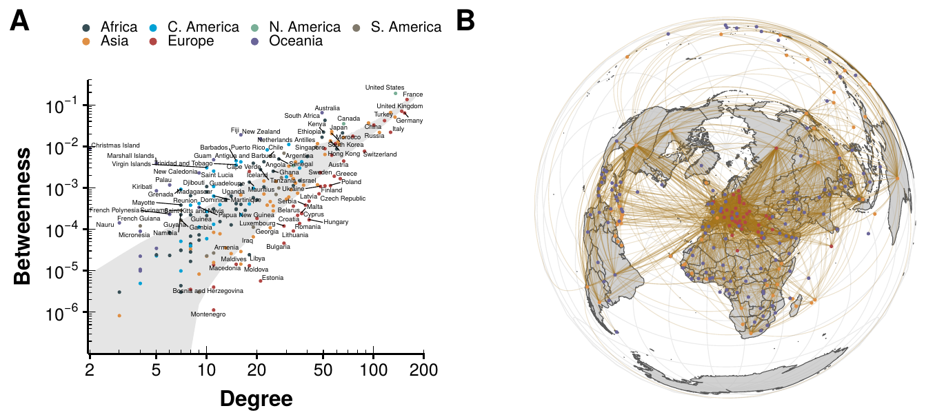
Figure 2.5: Analysis of the worldwide air transportation network with countries as nodes. In panel A we show the betweenness of each country in the network as a function of its degree. The shaded gray area represents where are 95% of the nodes belonging to \(10^4\) random graphs sampled from the ensemble. In other words, countries outside that region can be considered abnormal. Labels have been attached only to said countries. In panel B we show the geographical projection of the network, with those countries with betweenness higher than expected in orange and with those countries with lower values than expected in red.

In spite of all the methodological differences between our work and Guimerà et al. we do find a similar pattern of anomalies. For instance, Christmas Island is one of the countries with highest betweenness even though is the one with the lowest degree. Conversely, Montenegro, with degree 11, has one of the lowest values of betweenness. This clearly contradicts the results obtained for the graphs sampled from the ensemble built preserving, on average, the degree sequence of the network (shaded gray area). Indeed, in random networks the betweenness centrality tends to be proportional to the degree of the node.

Even more, using countries as nodes instead of cities reveals a clear pattern. We can see that most countries with betweenness below the expectation are European. On the other hand, most nodes laying above the expectation are islands. This can clearly be seen in figure 2.5B, where we show a representation of the network embedded in space. As we can see, Europe is much more densely connected that the rest of the world, due to having a large population shared in several countries. Thus, there are lot of connections between them that increase their degree but do not make them more central globally. The opposite effect is observed in islands and large countries, which act as bridges connecting either large territories or hardly accessible ones, increasing the number of shortest paths that go through them.

These observations also agree with our hypothesis. We expect that if weights - number of flights - are included in the network, the centrality of small, fairly disconnected islands will be reduced while the highly active airports in Europe will increase theirs. Thus, we will now add the number of flights between any two routes as weight. Note, however, that the calculation of shortest paths (the key ingredient of the betweenness centrality) tries to minimize the total weight of a path. Hence, a larger weight would make the connection less desirable, which is the opposite of what we want as a larger number of flights makes it easier to use that connection. For this reason, we will initially set the number of flights as weight, then we will randomize the network using the method presented in section 2.5.1 and, lastly, to compute the betweenness we will set the weights to be the inverse of the number of flights, i.e. \(w_{ij}'=w_{ij}^{-1}\). The results are shown in figure 2.6.

At first glance, we observe that the number of nodes in the betweenness plot is much smaller than before (figure 2.6A). The reason is that there are several nodes, both in the real network and in the randomized graphs, that have 0 betweenness. In other terms, there are not any shortest paths going through them. This was somehow expected given that in figure 2.5A there were several small countries which clearly do not have as many daily flights as the biggest hubs in the world, for instance the islands in Oceania. Nonetheless, now most islands are compatible with the randomized graphs, as well as most European countries.

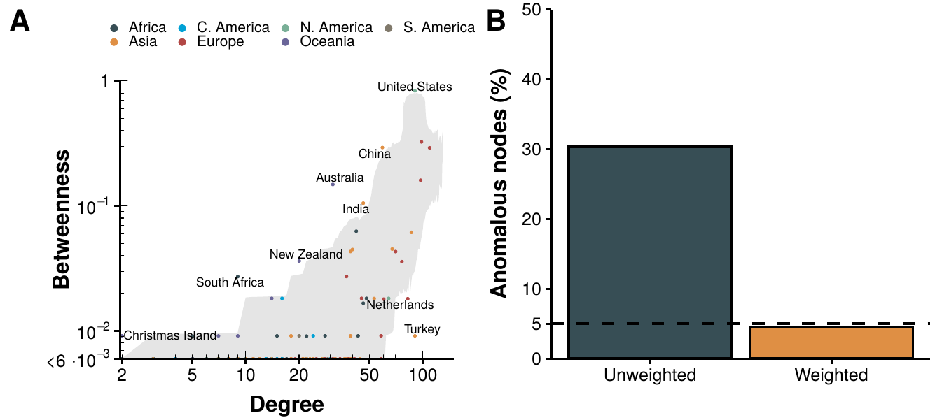
Figure 2.6: Analysis of the weighted worldwide air transportation network with countries as nodes. In panel A we show the betweenness of each country in the network as a function of its degree. The shaded gray area represents where are 95% of the nodes belonging to \(10^4\) random graphs sampled from the ensemble. Labels have been attached only to countries outside the expectation. In panel B we show the fraction of nodes that can be considered anomalous in the undirected network (left) and in the weighted network (right). The dashed line indicates the 5% threshold.

To facilitate the comparison of both approaches, in figure 2.6B we show the percentage of nodes that are not compatible with 95% of the randomized graphs. In the case of the undirected network, we find over 40% of nodes out of the area covered by the randomized graphs. Contrariwise, when weights are added to the network, the amount of anomalous nodes goes below the 5% mark. Thus, it is clear that the anomaly that was observed in the undirected case is solved once one considers weights. We will not try to answer why the weights are distributed the way they are, as it is probably a mixture of geographical, economical and political reasons, out of the scope of this analysis. Nevertheless, this result partially answers our initial question. Sometimes anomalies can be a byproduct of using a model that is simpler than it should be. To increase the validity of this statement, in the following section we will repeat the analysis on other types of transportation networks.

2.5.3 Other transportation networks

This analysis can be extended to other transportation networks. In particular, we have obtained the inter-city bus transportation networks of Brazil, Great Britain and Spain. Besides, we will now consider the full air transportation network, with cities as nodes, as in the work by Guimerà et al. [118]. The networks are represented in figure 2.7.

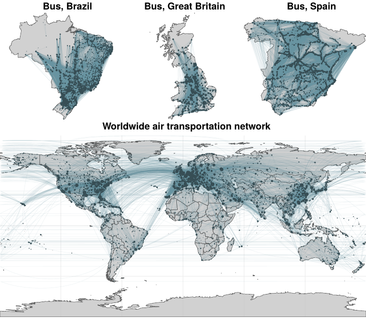
Figure 2.7: Spatial representation of transportation networks. The four networks under consideration are represented embedded in their corresponding spaces. Nodes are located in the center of their administrative region in the case of bus networks and in the coordinates of the city they belong to in the case of the air transportation network. The size of the nodes is proportional to their degree.

Data from the Brazilian inter-city routes was obtained from the Brazilian National Land Transportation Agency (ANTT) [126]. The data corresponds to the period between January 2005 and December 2014 with a monthly resolution and includes more than 19,000 unique routes connecting 1,786 cities. The geographical location of the nodes was determined using data from the Brazilian Institute of Geography and Statistics (IBGE) [127].

Similarly, data from the British inter-city routes was contained in the National Public Transport Data Repository (NPTDR) maintained by the Department of Transport. The data corresponds to the period between October 4, 2010 to October 10, 2010, with an hourly resolution. This dataset was complemented with the National Coach Services Data (NCSD) distributed also by the Department of Transport [128]. The total number of nodes is 279 nodes with almost 4,000 unique routes.

For the case of Spain, however, there is no public repository containing the data in a suitable format to be used. Thus, we had to scrap the data from a website maintained by the Spanish Ministry of Development that offers information of all the bus connections between municipalities in Spain except for the province of Girona [129]. The data corresponds to the period between January 1, 2017 and December 31, 2017. The total number of nodes is 1,435 with over 20,000 unique routes. As nodes in this network are municipalities instead of cities, we aggregated in all networks their bus stops into their corresponding municipalities.

Next, we repeat the analysis outlined in section 2.5.2 on these 4 networks. To sum up, we first build the unweighted version of the networks and randomize them using the formalism of undirected binary graphs presented in section 2.4.1. We then compare the betweenness of the real nodes to their randomized counterparts. If their betweenness is higher than their randomized versions in \(97.5\%\) of the samples, or if it is lower than in \(2.5\%\) of the samples, we flag them as abnormal nodes. We measure the amount of nodes that can be regarded as abnormal in all networks, and then repeat the whole process with the weighted versions of the networks, using the appropriate null model (section 2.5.1). The results are depicted in figure 2.8.

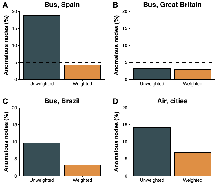
Figure 2.8: Fraction of anomalous nodes in transportation networks. Percentage of anomalous nodes in each network for the unweighted and weighted versions of the networks. The anomaly is verified for all unweighted networks, except for Great Britain. In contrast, in the weighted version the fraction of anomalous nodes is of the order of the false discovery rate, i.e., approximately 5%.

Several observations are in order. First, we not only find the expected anomalies in the worldwide air transportation network, but also in the Brazilian and Spanish bus networks. In the case of Great Britain we do not observe anomalies, although this network has some special characteristics that might explain this fact. Indeed, as we can see in figure 2.7 large cities are situated in the middle, with few small cities in the north and some more in the south. This centralization might explain why we do not see small nodes with large values of betweenness. Besides, municipalities are larger than in other countries and as a result the number of nodes in this network is one order of magnitude below the Spanish and Brazilian networks. This reduces the amount of unique routes and tends to centralize them, preventing routes in isolated areas that would increase the centrality of small nodes (which would actually be even smaller if we had not aggregated them). In any case, regardless of the specific reasons for this observation, it seems that for the particular case of the Great Britain network it is enough to consider only the degree of the nodes to avoid anomalies.

Nevertheless, in the weighted versions of the networks we can see that systematically the amount of anomalous nodes is reduced in all networks, even in the one from Great Britain (although both the weighted and unweighted amounts are below the 5% line and thus we cannot state that the reduction is significant). This result suggests that the existence of centrality anomalies in transportation networks might be a consequence of neglected, but functionally crucial, information about the system.

The exponential random graph framework allows us to build very general null models in which only the information we provide is fixed, the rest being maximally random. This is specially important when one wants to analyze if the characteristics of a real network are different from what would be expected from alike graphs. Indeed, if all the assumptions implicit in a null model are not under control, it is possible to find anomalies that might be just a byproduct of the null model itself, rather than coming from the real system.

In this particular case, we have seen that when one only gathers information about the degree of the nodes in a transportation network, their centrality does not behave as expected. However, by adding a small piece of information - the weight of the links - the network starts to behave as its random counterparts. Hence, this work highlights the fact that when some anomalies are found in a network, care must be taken in order to determine if those anomalies are really important or just a consequence of not using the proper amount of information.

Even more, we propose that this technique might be useful to determine how much data of a system is needed, or how complex its network model has to be. In the particular case of transportation networks the use of weights is rather straightforward. However, in systems in which the choice might not be so obvious, hunting for anomalies and looking for network characteristics that can explain them, might be the key to determine the most important elements of the system.

2.6 Generating data-driven contact networks

What about the children?!
Won’t somebody please think of the children!?
Helen Lovejoy

Contact networks are graphs whose nodes represent individuals and their links represent some kind of close interaction between them. This kind of networks are of particular interest in the field of epidemiology, as there are several diseases which can only be transmitted from person to person, such as influenza, tuberculosis or HIV. Thus, the contact patterns of the population can provide the necessary information to implement preventive measures . For instance, by analyzing who are the most central nodes in the network, it is possible to devise efficient vaccination strategies .

Yet, even for small populations, obtaining the whole contact network of the population is really hard. A prominent example can be found in the case of sexually transmitted diseases. It is clear that in those particular diseases it should be possible, in general, to trace back the whole chain of infections and, ideally, reconstruct the contact network . However, this process is full of biases, such as individuals not being willing to provide detailed information about their sexual partners . In practice, it is only possible to trace back the whole chain of infections for very small epidemic outbreaks .

Hence, to study large scale epidemics one usually resorts to building synthetic contact networks. In some cases, they can be based on some ad hoc assumptions specific for the disease under study . In others, a small portion of the population is thoroughly investigated and then its characteristics are extended to the whole population . Another possibility is to use aggregated statistics about the population such as household size or age distributions to build them . The framework that we will develop in the following pages will follow the latter.

One of the key elements defining contact networks is the social structure of the population. It has been observed that individuals have very different mixing patterns depending on their age, and even that they vary greatly from country to country . The usual approach to implement this in epidemic spreading models is to consider that the whole population is in contact with each other (resembling a fully connected graph) and weighting the transmission probability between two individuals according to their respective ages . This, however, completely neglects the network structure of the population.

In this work we propose a methodology to build contact networks based on the exponential random graph model using socio-demographic data. In particular, we will take into account the demographic structure of the population as well as their mixing patterns. As previously mentioned, these patterns are highly dependent on the age of the individual. Thus, age will be the key ingredient in this model. Besides, we will arrange individuals with similar age in layers, building a multilayer network. As we shall see in section this will facilitate the study of disease spreading on these networks. However, in this section we will only focus on the methodology used to build said networks.

2.6.1 Theoretical framework

Demographic studies usually classify individuals into age groups, also known as age brackets, instead of using their exact value. Hence, mixing patterns are often given in the form of number of contacts between individuals in age group X with individuals in age group Y. For this reason, we will consider that the population is divided into \(L\) layers, one for each age group. The number of nodes in each layer will be set according to the demographic structure of the population under study. We will denote by \(n_\alpha\) the set of individuals contained in layer \(\alpha\) or, equivalently, with age contained in age bracket \(\alpha\) (henceforth, individual with age \(\alpha\)). Thus, the total number of nodes will be \(N = \sum_{\alpha=1}^L |n_\alpha|\).

Besides the demographic structure of the population, we will suppose that the only information we have is the number of (undirected) links of individual \(i\) in layer \(\alpha\) to individuals in layer \(\beta\). As a consequence, the quantity that we want to preserve is the layer-to-layer degree, \(k_{i,\alpha}^\beta = \sum_{j\in n_\beta} a_{ij}\) (the procedure to extract this information from real data will be described in section 2.6.2). An schematic representation of the system is depicted in figure 2.9.

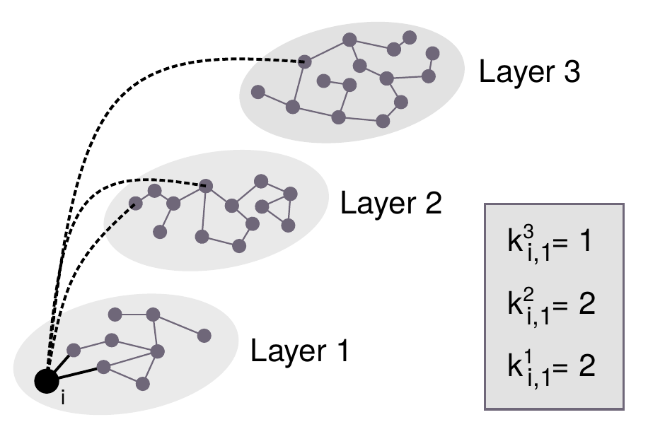
Figure 2.9: Schematic of a multilayer network with age-dependent contacts. Each layer represents one age bracket \([a_\text{lmin},a_\text{lmax})\), so that individuals set in layer \(l\) are between \(a_\text{lmin}\) and \(a_\text{lmax}\) years old. Links can be inside layers, representing contacts with individuals within the same age bracket, and across layers, representing contacts with individuals of different age. For instance, node \(i\) has two links in layer 1, two links to layer 2 and one link in layer 3 so that \(\{k_{i,\alpha}^{\beta}\} = \{k_{i,1}^\beta\} = \{2,2,1\}\).

Under these assumptions, the Hamiltonian of the graph reads

\[\begin{equation} H(G,\theta) = \sum_{\alpha=1}^L \sum_{\beta=1}^L \sum_{i\in n_\alpha} \theta_{i,\alpha}^\beta k_{i,\alpha}^\beta\,, \tag{2.56} \end{equation}\]

which can be rewritten in a more useful way after some algebra,

\[\begin{equation} \begin{split} H(G,\theta) & = \sum_{\alpha=1}^L \sum_{\beta=1}^L \sum_{i \in n_\alpha} \theta_{i,\alpha}^\beta \sum_{j \in n_\beta} a_{ij} = \sum_{\alpha=1}^L \sum_{i \in n_\alpha} \sum_{j=1}^N \theta_{i,\alpha}^\beta a_{ij} \\ & = \sum_{i=1}^N \sum_{j=1}^N \theta_{i,\alpha}^\beta a_{ij} = \sum_{i<j} (\theta_{i,\alpha}^\beta + \theta_{j,\beta}^\alpha) a_{ij} \,. \end{split} \tag{2.57} \end{equation}\]

In the derivation of equation (2.57) we have used the fact that node \(i\) only belongs to layer \(\alpha\). This is not the case in general multilayer networks, where one node can be present in more than one layer. However, in this particular case, as an individual can only have one age, it can only belong to one layer. Note that this also implies that this problem can be mapped into the one of building single layer exponential random graphs with fixed community structure and degree sequence [130].

Now, the probability of finding any graph \(G\) in the ensemble will be

\[\begin{equation} \begin{split} P(G|\theta) & = \frac{e^{-\sum_{i<j} (\theta_{i,\alpha}^\beta + \theta_{j,\beta}^\alpha) a_{ij}}}{\sum_G e^{-\sum_{i<j} (\theta_{i,\alpha}^\beta + \theta_{j,\beta}^\alpha) a_{ij}}} = \prod_{i<j} \frac{\left(e^{-\theta_{i,\alpha}^\beta} e^{-\theta_{j,\beta}^\alpha}\right)^{a_{ij}}}{1+e^{-\theta_{i,\alpha}^\beta} e^{-\theta_{j,\beta}^\alpha}} \\ & = \prod_{i<j} \frac{(x_{i,\alpha}^\beta x_{j,\beta}^\alpha)^{a_{ij}}}{1+x_{i,\alpha}^\beta x_{j,\beta}^\alpha} = \prod_{i<j} p_{ij}^{a_{ij}} (1-p_{ij})^{1-a_{ij}}\,, \end{split} \tag{2.58} \end{equation}\]

where, similarly to previous sections, we have defined the auxiliary variable \(x_{i,\alpha}^\beta \equiv e^{-\theta_{i,\alpha}^\beta}\) and the probability of having a link between node \(i\) and \(j\) as

\[\begin{equation} p_{ij} \equiv \frac{x_{i,\alpha}^\beta x_{j,\beta}^\alpha}{1+x_{i,\alpha}^\beta x_{j,\beta}^\alpha}\,. \tag{2.59} \end{equation}\]

Note that the shape of equation (2.58) is equivalent to the one of undirected binary networks, section 2.4.1. Hence, to sample networks from this ensemble we can simply perform sequential Bernoulli trials on each pair of nodes.

Lastly, to obtain the value of \(x_{i,\alpha}^\beta\) we only need to maximize the log-likelihood which in this case reads

\[\begin{equation} \begin{split} \mathcal{L}(\theta) & = \ln \prod_{i<j} p_{ij}^{a_{ij}}(1-p_{ij})^{1-a_{ij}} \\ & = \sum_{i=1}^N \sum_{j=i+1}^N a_{ij} \ln \frac{x_{i,\alpha}^\beta x_{j,\beta}^\alpha}{1+x_{i,\alpha}^\beta x_{j,\beta}^\alpha}+ (1-a_{ij}) \ln \frac{1}{1+x_{i,\alpha}^\beta x_{j,\beta}^\alpha} \\ & = \sum_{i=1}^N \sum_{j=i+1}^N a_{ij} \ln (x_{i,\alpha}^\beta x_{j,\beta}^\alpha) - \ln(1+x_{i,\alpha}^\beta x_{j,\beta}^\alpha) \\ & = \sum_{i=1}^N \sum_{\beta=1}^L k_{i,\alpha}^\beta \ln x_{i,\alpha}^\beta - \sum_{i=1}^N \sum_{j=i+1}^N \ln(1+x_{i,\alpha}^\beta x_{j,\beta}^\alpha) \,. \end{split} \tag{2.60} \end{equation}\]

Thus, the process is analogous to the one we have seen in sections 2.4.1, 2.4.2 and 2.5.1. Indeed, once the constraints have been established, we need to maximize the log-likelihood to obtain the appropriate values of \(\theta_{i,\alpha}^\beta\). Then, we can get the probability of two nodes being connected from equation (2.59). Lastly, we can perform measurements over the whole ensemble using the full \(P(G|\theta)\) or sample networks using independent Bernoulli trials on each pair of nodes. In the following section we will describe how we can obtain the values of the constraints, \(k_{i,\alpha}^\beta\), from real data.

2.6.2 Data description

The key ingredient of the proposed methodology is the number of links a node \(i\) has within its layer, \(\alpha\), and to each of the other layers, \(\beta\), denoted as \(k_{i,\alpha}^\beta\). In order to generate realistic distributions of this quantity, we would need the probability distribution of a node with age \(a\) to contact \(k\) individuals of age \(a'\), \(P(k,a,a')\). Fortunately, there are some empirical studies that provide enough information to do so, such as the POLYMOD study [131].

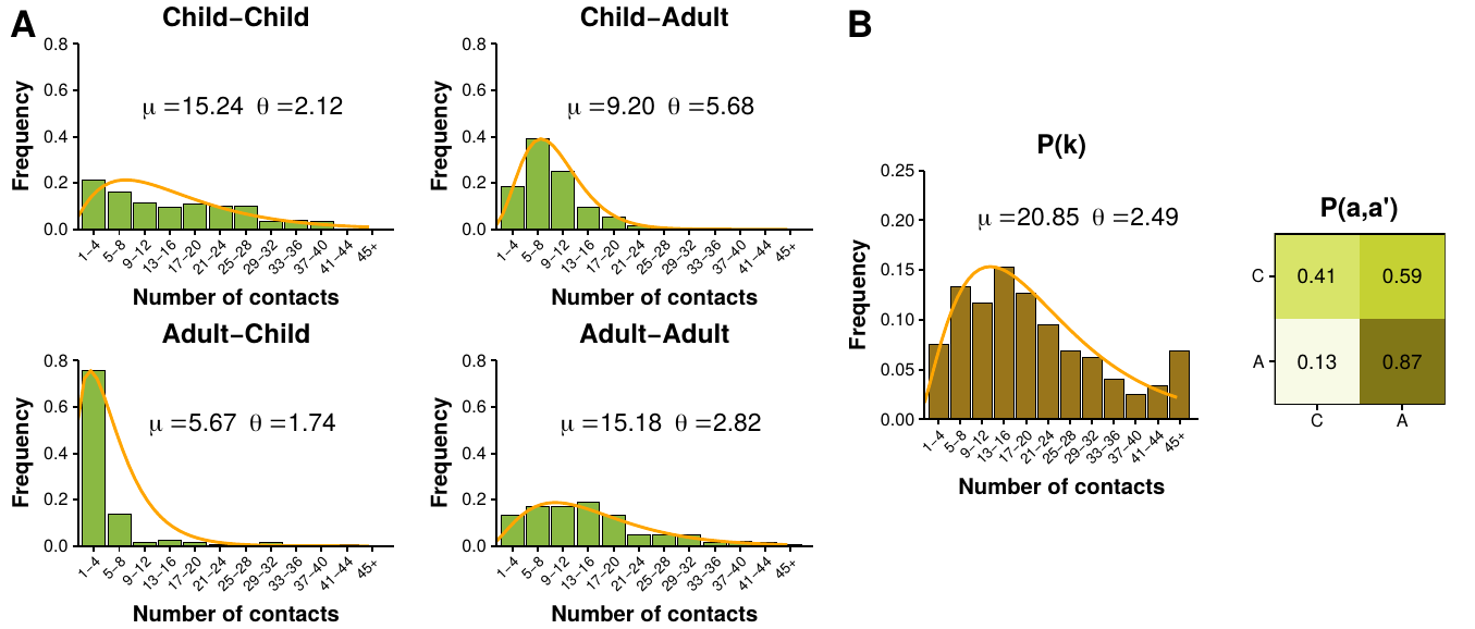
Figure 2.10: Mixing patterns of the Italian population. The population has been divided into two groups: children (individuals aged 18 or less) and adults (individuals aged 19 or more). In A the distribution of the number of contacts between the different groups is shown. The fitted curve corresponds to a negative binomial distribution parameterized with mean \(\mu\) and shape \(\theta\). In B the total number of contacts, regardless of the age of the individual, is shown. As in A, the fitted curve corresponds to a negative binomial distribution. Besides, the matrix on the right represents the probability that an individual in age group \(a\) (rows) contacts with an individual in age group \(a'\) (columns).

In the POLYMOD study volunteers from eight different European countries were asked to provide information about who they contacted during a given period of time. In particular, the information that is relevant for our interests is the age of the participant, \(a\), and the age of the person contacted, \(a'\). Then, aggregating this data, we can obtain the distribution of the number of contacts that an average person of age \(a\) has with people of age \(a'\), \(P(k,a,a')\). In figure 2.10A we show this distribution for the case of Italy, which was one of the most complete surveys of the study.

To facilitate the visualization of the results, we have chosen to classify individuals, following previous literature [132], into two age groups: children (aged 18 or less) and adults (aged 19 or more). Then, we have measured the number of contacts each child had with other children (top-left distribution) and with adults (top-right distribution). Similarly, on the bottom row we show the contact distribution of adults with children (bottom-left) and of adults with other adults (bottom-right). All empirical distributions have been fitted to a negative binomial distribution, which is one of the most common methods for analyzing count response surveys⁷ [133].

However, this data has some drawbacks, such as the problem of reciprocity. In a completely closed population (and with perfect measurement instruments), for each contact that a child reports with an adult we should get a report of and adult contacting a child. But, as in this survey the population was not closed, that is, people participating in the survey could report contacts with people not participating in it, the reciprocity condition is not always satisfied. This is a well known problem in the study of mixing patterns of the population and there are several techniques used to solve it, such as the pairwise correction [134]. Thus, we will perform an assumption that will allow us to leverage all the techniques that have already been developed to work with age-contact matrices.

Indeed, from now on, we will suppose that the probability of having \(k\) contacts is independent of the age of both individuals involved in it. That is, \(P(k,a,a') \approx P(k) P(a,a')\). Note that with this assumption we have separated the mixing patterns of the population, \(P(a,a')\), from the main topological characteristic of networks, the degree distribution \(P(k)\). This has two main advantages. First, this will allow us to directly input into the model mixing contact matrices, which are more common in the literature than the whole survey data. Second, we will be able to test the effect of different degree distributions. This situation will be further analyzed in section 3.4.

In figure 2.10B we show the necessary information to build \(P(k,a,a')\) under this assumption. As we can see, the average number of contacts of any individual in the Italian population is close to 21. Interestingly, this number can vary greatly. For instance, while Italy was the country with the highest number of reported contacts, Germany was the one with the fewest daily contacts, 8. Regarding \(P(a,a')\), it is important to note that the matrix is not symmetric per se, but this is due to the fact that age groups are not equally sized. Indeed, if we suppose that all groups have the same degree distribution, the reciprocity condition implies that \(N_a P(a,a') = N_{a'} P(a',a)\), where \(N_a\) represents the number of individuals with age \(a\).

Summing up, to obtain \(k_{i,\alpha}^\beta\) we simply need to sample \(k\) from the desired degree distribution for each node \(i\) of age \(\alpha\). Then, we can distribute this value across layers using a multinomial distribution with probability parameters \(P(\alpha,\beta)\).

2.6.3 Age contact networks

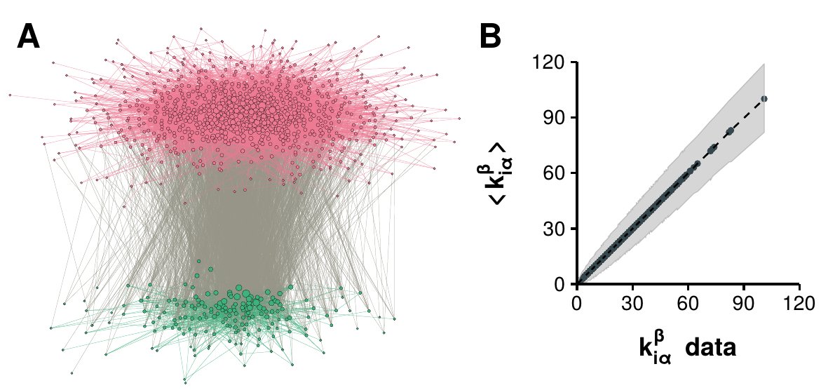
Figure 2.11: Synthetic Italian age contact network. A) depicts a random network obtained from the ensemble. The size of the nodes is proportional to their degree. The layer on the bottom corresponds to nodes classified as children, while the layer on top corresponds to adults. The difference in group size is due to the demographic structure of the country. B) Comparison of the average degree of each node obtained from averaging \(10^4\) networks sampled from the ensemble to the imposed constraint. The 95% confidence interval of the distribution is shown in gray for each node.

We will finish this section demonstrating the full process of generating one age contact network, which can be divided in three steps:

1. Data collection and standardization: the first step is to obtain demographic structure, mixing patterns and degree distribution of the population under consideration. Standardization in this context refers to deciding the number of age groups in the system and modifying the distributions accordingly.

As in the previous section, we will focus on Italy in the year 2005, which is when the POLYMOD study took place. Besides, we will consider that there are still only two groups, children and adults. Under these circumstances, according to the demographic structure of the country, \(18\%\) of the nodes must be set in the age group of children while the other \(82\%\) must belong to the adults group. The \(P(a,a')\) matrix as well as the degree distribution will be the ones shown in figure B.

Next, we need to decide the number of nodes in our network. In this case, we will set this number equal to \(N=10^3\). Hence, there will be 180 nodes and 819 nodes in layers 1 and 2 respectively. Once this is set, we can extract suitable values of \(k_{i,\alpha}^\beta\) for each node \(i\) from the \(P(k,a,a')\) distribution as explained in the previous section. These will be the constraints in our model.

2. Determination of the ensemble: once the constraints are set, the next step is to maximize the log-likelihood defined in to obtain the proper values of \(x_{i,\alpha}^\beta\). These can be used to build the ensemble of networks using (2.58).

3. Network sampling: the last step is to randomly sample as many networks as desired from the ensemble. This can be easily done by performing a Bernoulli trial over each pair of nodes \(i\) and \(j\) with probability of success given by \(p_{ij}\) as defined in equation (2.59).

For this example, we have sampled \(10^4\) networks from the ensemble. In figure 2.11A we show one of the sampled networks. As it can be seen, the network is divided in two layers. Nodes in the bottom layer represent children while the ones on top adults. As imposed by the demographic constraints, there are many more nodes in the adults layer than in the children layer. To confirm that the sampled networks successfully preserve the rest of the constraints, in figure 2.11B we plot the average value of \(k_{i,\alpha}^\beta\) in the set of \(10^4\) networks (\(y\) axis) against the value imposed by the data (\(x\) axis). Clearly, all nodes are close to the identity line, indicating that the conditions were successfully maintained.

This example demonstrates that we now have all the tools required to generate realistic contact networks with age related data. In section 3.4 we will use this framework to build networks for different countries and periods of time, and we will measure the impact that incorporating this kind of data can have on disease dynamics.

---

7. Count data is usually modeled in physics as a Poisson distribution, whose mean equals its variance. In count data involving humans, however, this is not usually the case. Thus, negative binomial distributions are used instead, as their variance can be larger than the mean. This special characteristic of these distributions is known as overdispersion.↩︎