Computational Physics
In this course we teach various computational techniques and their applications in solving physical problems using the C programming language.
In 2024, we introduced a new way of teaching the practical part of the course, using complex and (hopefully) interesting/funny problems that require the application of multiple techniques learned throughout the course, including tools such as GitHub. To facilitate this, we provide automated tests to help students verify the correctness of their implementations through GitHub Classroom.
In this page you can find links to these assignments and some visualizations created by the students.
2023/2024 Projects
Project 1: Harmonic Oscillator
Description: Simulate the motion of an harmonic oscillator using numerical integration methods.
Techniques Used: Euler method and Verlet integration.
Link to Code: GitHub Repository
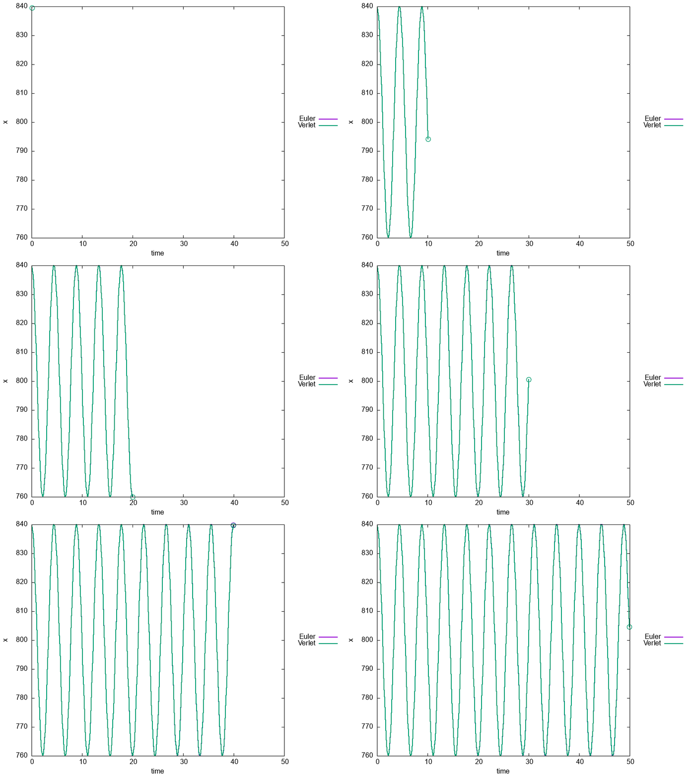
Since this was the first assignment ever and we weren’t sure if students would be able to work with GitHub and Visual Studio Code, we kept it simple. The goal was to implement two numerical integration methods (Euler and Verlet) to simulate the motion of a harmonic oscillator and compare their accuracy. Later on, in the exam, we asked them to add small modifications to their code, such as a slighlty different potential.
Project 2: Brownian Motion
Description: Simulate the Brownian motion of a student who may have drunk a bit more than they should in a 2D grid, avoiding obstacles and trying to get to class on time.
Techniques Used: Random number generation, Monte Carlo methods, and collision detection.
Link to Code: GitHub Repository
For this second project, we wanted to introduce random number generation and Monte Carlo methods. The task was to simulate a student moving in a 2D grid, where they could randomly move in different directions, but had to avoid obstacles (like buildings) and try to reach their class on time. This project required students to implement collision detection and use random numbers to determine the student’s movement.
2024/2025 Projects
Project 1: Solar System
Description: Simulate the motion of planets in a solar system using numerical integration methods.
Techniques Used: Verlet integration, gravitational forces, and data visualization.
Link to Code: GitHub Repository
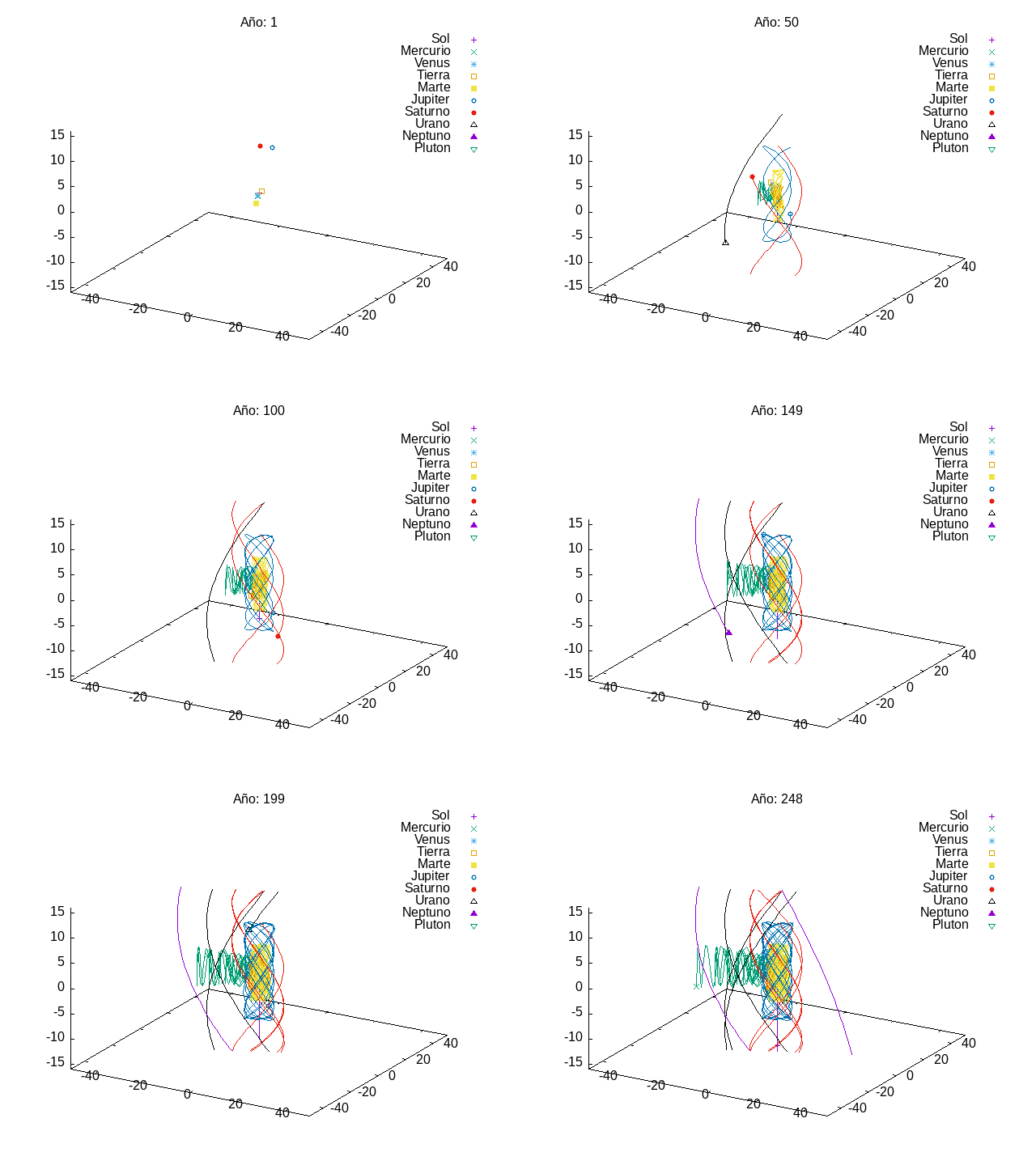
This year, given the success of last year’s projects, we increased slightly the complexity of the first project. In this case, they had to simulate a solar system with multiple planets orbiting a star. We know that integrating a system of coupled differential equations is always a bit tricky and, actually, many students struggles a bit with it:
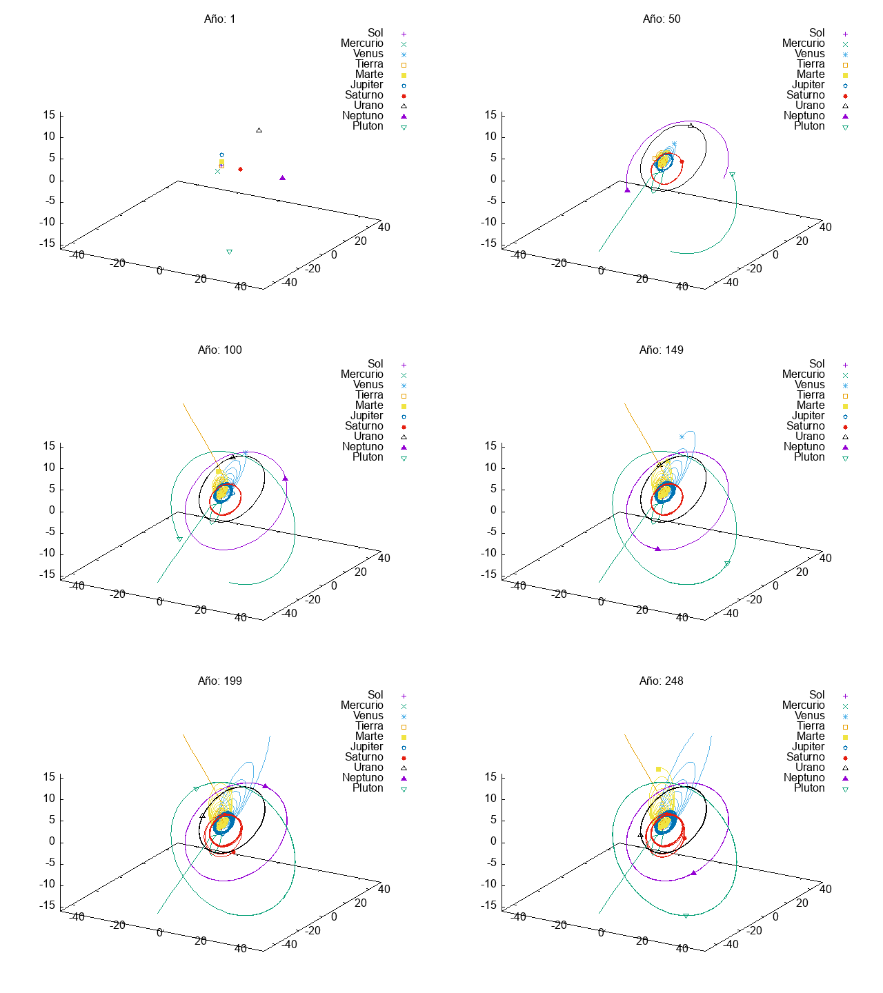
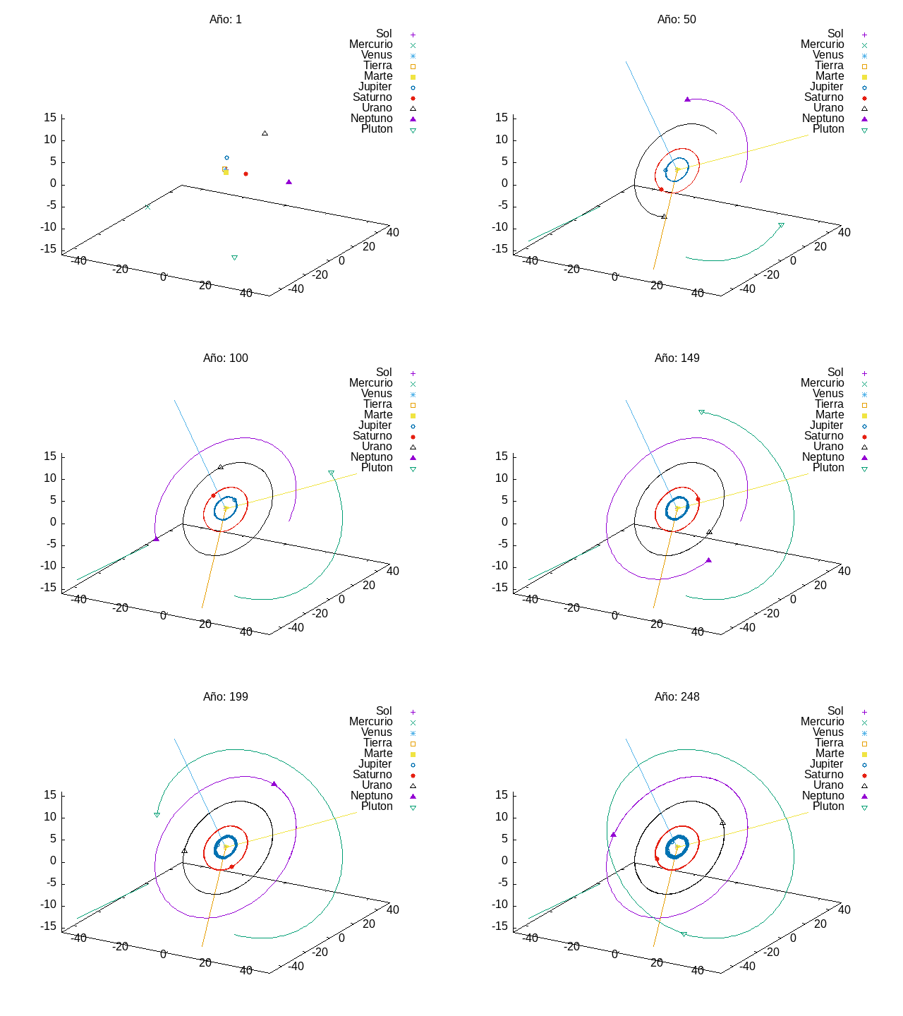
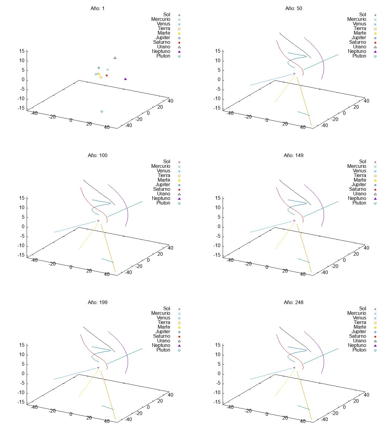
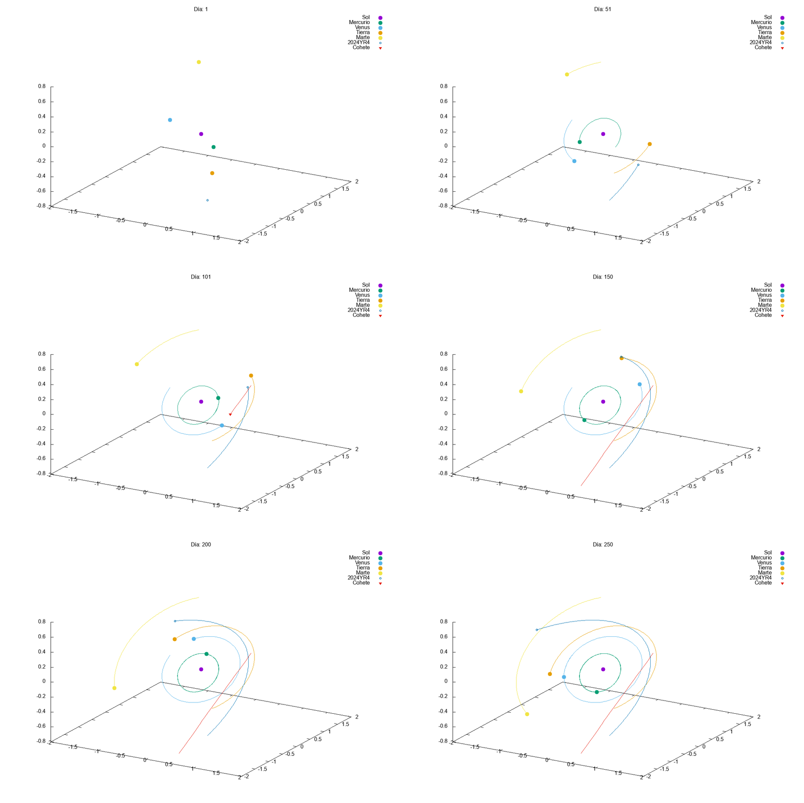
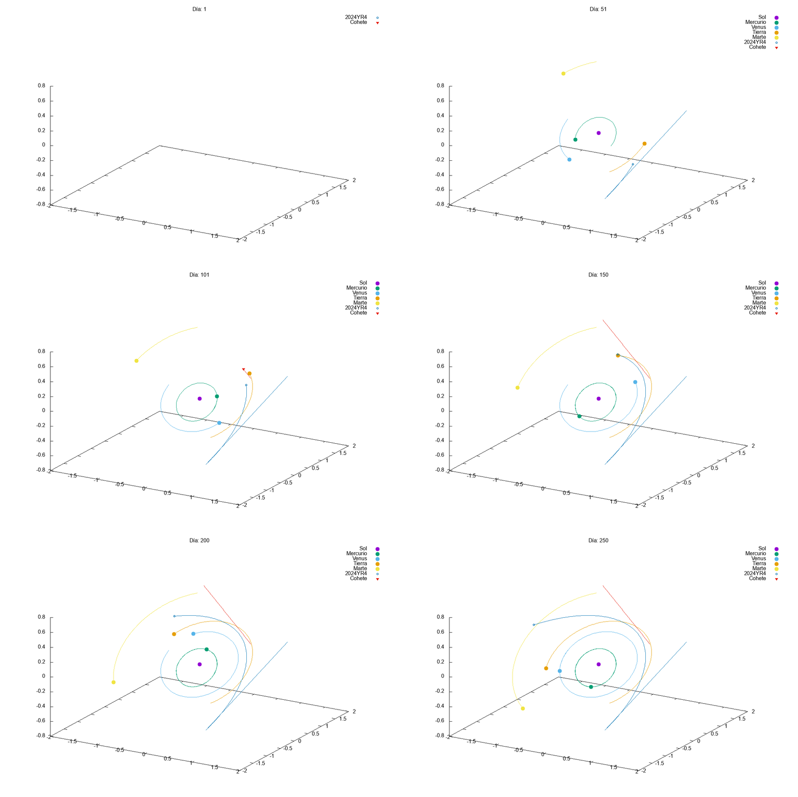
Then, in the exam, we asked them to add small modifications to their code, so that they could divert the orbit of an asteroid that was going to hit the Earth (Armageddon style). Let’s just say that we need to find better pilots for our future space missions…


Project 2: Rumba
Description: Simulate the movement of a robot vacuum cleaner (Rumba) in the first floor of the Faculty of Science, using random walk and collision detection.
Techniques Used: Random number generation, Monte Carlo methods, collision detection, and videogame physics.
Link to Code: GitHub Repository
For the second project, we wanted to introduce a bit of videogame physics, so instead of generating some data and then visualizing it, we set up a simple 2D videogame-like environment using the SDL3 library. This allowed them to see their code in action, as they could see the Rumba moving around the floor, avoiding obstacles and cleaning the area.
In the exam, we asked them a very short question and allowed them to use any resources they wanted (including internet, chatGPT, books, classmates, etc.): “What Rumba should we buy? Justify your answer.”
Let’s just say that they weren’t ready for such a difficult question…
Other Resources
- [In Spanish] Los malditos punteros: notes from the 2018/2019 Computational Physics course at the University of Zaragoza on the functioning of pointers in C.